Unravelling Urban Pedestrian Trips

Transcription

1

2 ii

3 Unravelling Urban Pedestrian Trips Developing a new pedestrian route choice model estimated from revealed preference GPS data By R.E. Hintaran in partial fulfilment of the requirements for the degree of Master of Science in Transport, Infrastructure and Logistics at the Delft University of Technology, to be defended publicly on Monday January 4th, 2016 at 14:00 PM. Graduation committee: Chair: Prof. dr. ir. S.P. Hoogendoorn TU Delft Dr. ir. W. Daamen TU Delft Dr. J.A. Annema TU Delft External Supervisors: Prof. dr. K.W. Axhausen ETH Zürich L. Montini, MSc ETH Zürich An electronic version of this thesis is available at iii

4 iv

5 Preface This thesis shows the results of my graduation project on pedestrian route choice behaviour in urban areas. It is fulfilled as part of the master program Transport, Infrastructure and Logistics at Delft University of Technology. The graduation project was carried out in cooperation with ETH Zürich. However, it would be possible to be accomplished without the guidance and support of several people. Therefore, I would like to thank all the people who have supported me during my graduation project. First of all, I would like to thank my daily supervisor at TU Delft, Winnie Daamen, for her scientific and personal support throughout the entire project. She was always critical and realistic, but also understanding when it was needed. It often happened that I was lost in my thesis work, but Winnie always knew how to motivate me with sharp feedback. I enjoyed the many thesis and off-thesis discussions that we had, and it was very inspiring to work with such a committed scientist. Secondly, I would like to thank my second daily supervisor at TU Delft, Jan Anne Annema, for his scientific support and his infinite optimism and enthusiasm. His encouraging feedback and positive spirit helped me to structure my work and to see the greater picture. Lastly, I would like to thank Serge Hoogendoorn for his encouragement, support and his natural enthusiasm for this topic. His contagious enthusiasm and bright ideas motivated me to find new solutions. I would also like to thank Prof. Kay Axhausen for inviting me to his institute, for his support during my thesis and for giving me the freedom to define my own research project at the institute. Furthermore, I would like to thank Lara Montini, my daily supervisor at ETH Zürich, for her guidance during my time in in Zürich and for her patience to learn me programming in Java. She was always very patient and helpful, even when I was already back in the Netherlands. Also, I would like to thank my colleagues at ETH Zürich for the great and unforgettable time. In the four months that I spent there I have learned a lot of things and I got the opportunity to join my colleagues to the yearly Swiss Transport Research Conference. Lastly, I would like to thank my friends for the fun times during my graduation project and all the other afstudeerders of the famous Afstudeerhok for fun times and fruitful discussions during coffee and lunch breaks and also outside the university. Special thanks go out to my parents and my sister, who were always supportive and who were always there for me. And also very special thanks to Eelco, for his unconditional support in all times and for always cheering me up with his positive perspective on life. Delft, December 2015 Eka Hintaran v

6 vi

7 vii

8 Contents Introduction Problem analysis Conceptual framework and research objective Contribution to practice Contribution to science Research approach Scope and research limitations Thesis outline... 9 State-of-the-art on Pedestrian Route Choice Behaviour Pedestrian route choice behaviour Route choice decision-making Environmental street characteristics influencing route choice behaviour Conclusion State-of-the-art on Pedestrian Route Choice modelling Observed routes Data collection methods RP studies in pedestrian research Generation of alternative routes Choice Set Generation in modelling process Requirements for the choice sets and the method Evaluation methods Different procedures Formulation of correlation structure Conclusion Case study Zürich Used data Street network Observed routes GPS data collection and post-processing Processing of GPS data Map-matching procedure Generation of alternative non-chosen routes Calculation of route characteristics and Path-Sizes Environmental street characteristics Path-Size factors (overlap) Writing final results for choice modelling Analysis of GPS and generated data Research plan Descriptive analysis of results Comparing the chosen routes with the alternative non-chosen routes in the choice set Conclusion Estimation of route choice models Research plan Model specification Basic Model Independent estimation of parameters Basic model results viii

9 6.3.3 Conclusion and next steps Sampling of alternatives Samples Sample of longest routes Random sample Importance Sampling Importance Sampling Conclusion data set Basic model Importance Sampling Conclusion Final Conclusion Conclusions and recommendations Findings Conclusions Recommendations for science and further research Recommendations for practice Discussion Bibliography Appendix 1 Study area in MATSim format and in OpenStreetMap Appendix 2 Example of Travel Diary Appendix Descriptive analysis chosen routes Appendix Model estimation results of sample of longest routes ix

10 List of Tables Table 1: Overview of route attributes that form the route characteristics Table 2: Overview of model formulations applied to slow modes Table 3: Overview of RP studies in pedestrians' research Table 4: Calculated Route Attributes Table 5: Characteristics of chosen routes Table 6: Descriptive analysis of all chosen routes Table 7: Descriptive analysis of non-chosen routes Table 8: Chosen route compared with alternative routes Table 9: Shortest routes and detours Table 10: Correlations between attributes for 20 and 21-data sets Table 11: Route class definition Table 12: Basic model with 20 alternatives, attributes independently estimated Table 13: Basic model PSL results, trip length in Distance (km) Table 14: Basic model PSL results, trip length in Route Classes Table 15: Random sample, attributes independently estimated Table 16: Random sample PSL results, trip length in Distance (km) Table 17: Random sample PSL results, trip length in Route Classes Table 18: Importance Sampling 1, attributes independently estimated Table 19: Importance Sampling 1 PSL results, trip length in Distance (km) Table 20: Importance Sampling 1 PSL results, trip length in Route Classes Table 21: Importance Sampling 2, attributes independently estimated Table 22: Importance Sampling 2 PSL results, trip length in Distance (km) Table 23: Importance Sampling 2 PSL results, trip length in Route Classes Table 24: Basic model 21-data set, attributes independently estimated Table 25: Basic model 21-data set PSL results, trip length in Distance (km) Table 26: Basic model 21-data set PSL results, trip length in Route Classes Table 27: Importance sampling 21-data set, attributes independently estimated Table 28: Importance Sampling 21 PSL results, trip length in Distance (km) Table 29: Importance Sampling 21 PSL results, trip length in Route Classes Table 30: Basic model and Importance Sampling 1 PSL results, trip length in Route Classes. 95 x

11 List of Figures Figure 1: Route selection scheme... 5 Figure 2: Basic Conceptual Framework... 6 Figure 3: Research approach and thesis outline... 9 Figure 4: Examples of overlapping and crossing routes (Bovy & Stern, 1990) Figure 5: Three different choice situations (Bovy & Stern, 1990) Figure 6: From objective to subjective factors Figure 7: Overview of the Route Choice Modelling process Figure 8: The overlapping Path problem (Ramming, 2002) Figure 9: Hierarchy in choice sets, from the pedestrian's and the researcher's perspective (Hoogendoorn-Lanser & van Nes, 2004) Figure 10: Overview of Choice Set Generation Methods Figure 11: Updated Conceptual Framework Figure 12: Extensive public transport network of Zürich ( 39 Figure 13: Study Area (left: right: constructed network (MATSim, visualised in VIA) Figure 14: Example of observed routes of one person (ArcGIS, using OSM network) Figure 15: Example GPS tracks and GPS device Figure 16: Comparison of GPS data with data from Mikrozensus 2010 (mode share and trip purpose) Figure 17: Visualisation of observed routes by one person before processing of GPS data (ArcGis, using OpenStreetMap network) Figure 18: Processing of GPS data Figure 19: Map-matching of GPS points Figure 20: GPS points (red) and walking trips after Map-Matching (green) Figure 21: Order in which the nodes are explored (stackoverflow.com) Figure 22: BFS-LE algorithm: d = depth; Sn = additional alternatives found at depth n; S = size of the choice set; b(d) = Number of candidate networks at depth d; (Rieser-Schüssler (2012)) Figure 23: Road types in the street network (visualisation in VIA) Figure 24: Overview of route attributes calculation Figure 25: Histogram of trip lengths in KM of chosen routes Figure 26: Distribution of walking trips by activity type Figure 27: Route from tram station to viewpoint in Open Street Map Figure 28: Route from tram station to viewpoint in VIA (left) and links used by alternative routes (right) Figure 29: Trip from the Polybahn to the Main station in Open Street Map Figure 30: Chosen trip in VIA Figure 31: Links used by alternative routes, in VIA Figure 32: Distribution of chosen routes ranked by distance (in percentage and counts) Figure 33: Route classes grouped by distance Figure 34: Frequency tables of 20-data set (left) and 21-data set (right); distribution of chosen routes ranked by distance Figure 35: Route classes grouped by distance (20-data set) Figure 36: Route classes grouped by distance (21-data set) Figure 37: Histogram of distances (20-data set) Figure 38: Histogram of distances (21-data set) Figure 39: Trip distances of two choice sets of 20-data set (left chosen is 0,09; right 0,16).. 68 xi

12 Figure 40: Trip distances of two choice sets of 21-data set (left chosen is 0,11; right 0,08).. 68 Figure 41: Overview of model estimations Figure 42: Central ( 102 xii

13 xiii

14 xiv

15 Executive summary Walking is very important in our lives: for millions of years, walking has been the most basic mode of transport. However, much less research has been done on walking and pedestrians compared to motorised vehicular modes. Especially pedestrian s route choice behaviour is an interesting topic in research. Knowledge about pedestrian s route choice behaviour is sparse, while this knowledge is very relevant for planning and designing public spaces (rail stations, airports) and pedestrians facilities in cities. Theory on pedestrian route choice behaviour could also support in planning and managing large events. Current trends and challenges, such as the growing world population and increasing urbanisation (both resulting in increasing pressure on urban space and its infrastructures), make this topic more and more important. Therefore, the objective of this thesis is to determine which environmental street characteristics have on influence on the route choice process. This choice process is influenced by various factors, but this thesis focuses on environmental street characteristics. The aim of this thesis is reflected in the main research question: Which environmental street characteristics have an influence on pedestrian route choice behaviour in urban areas? A literature review and a case study have been carried out to answer this main research question. The city of Zürich is taken as a case study for a revealed preference experiment and the data are collected by GPS trackers. The purpose of this thesis is to estimate a pedestrian route choice model based on revealed preference GPS data. Literature shows that pedestrians make choices on three levels: strategic level (departure time choice and activity pattern choice), tactical level (activity scheduling, activity area choice and route-choice to reach activity areas) and operational level (walking behaviour). The focus in this thesis is on the tactical level: route-choices from origin to destination. It is assumed that pedestrians mainly make their route choices simultaneously: he or she makes a choice for the entire route before departing and does not change it on the way. Which route is chosen is based on their perceptions of the transport network and on personal characteristics. When utility maximization is assumed, individuals choose, or intend to choose, the alternative with the highest perceived utility. Route choice behaviour of pedestrians is influenced by various factors: network characteristics, route characteristics, personal characteristics and trip characteristics. A fifth category that also influences route choices are circumstances, such as weather conditions and traffic information. Environmental street characteristics belong the route characteristics category. Literature study on pedestrian route choice behaviour in urban areas shows that trip length is in most of the cases the most dominant factor in route choices. Other reported influential factors are scenery and safety factors, but these are not directly measurable from the network thus not taken into account in this thesis. Other selected attributes are road type and gradient, as road type relates with safety factors and comfort and gradient is related to physical effort, and especially important in a hilly city such as Zürich. Both environmental street characteristics are measurable from the available network. Pedestrian route choice modelling As the aim of this thesis is to report a pedestrian route choice model estimated on the basis of revealed preference data, first the suitable methods for each step in the route choice modelling process was selected. The route choice modelling process consists of three main steps: obtaining trip observations, xv

16 generating alternative non-chosen routes and defining the correlation structure between the alternatives in the choice set. These steps are essential before the actual estimation process could start. In this thesis, utility maximization is assumed, thus route choice behaviour is described within the discrete choice modelling framework. The main idea of utility maximization is that individuals make a subjective rational choice between a finite number of choice options and select the alternative with the highest utility. As revealed pedestrian s route choices in an urban area is modelled, the selected model formulation needs to be able to work with a dense real size network, to handle the extensive data set and to account for similarities in alternatives (overlap). The best option for the situation in this thesis turned out to be the Path-Size Logit model: it is able to capture overlap among routes, it is known to be sufficiently robust, it has the relatively simple MNL structure and it has been shown to perform well relative to more complex model forms in real size networks. For route choice modelling, both observed trips as non-chosen alternative trips are required. These two form the choice set. In this revealed preference study, trip observations are collected using GPS technology. The non-chosen alternative routes are generated using the Breadth First Search on Link Elimination (BFS-LE) method. This algorithm has proven to be efficient and consistent in bicycle route choice studies using large urban networks, and it has computational speed. Also, the BFS-LE method enables to use any (multi-attribute) cost-function so environmental factors can be taken into account when generating the routes. Furthermore, the method has shown to be able to generate heterogeneous routes. Choice set generation is a very complex task, as the analyst lacks information about the exact alternatives that are known and considered by the traveller. The last step was to define the correlation structure between the alternatives in the choice set. As mentioned earlier, the Path-Size Logit model is selected to describe pedestrian s route choices. In order to use a Path-Size Logit model, the adjustment term (Path-Size Factor) needs to be defined and calculated for each choice set. There are several Path-Size Factor formulations proposed, the challenge is to select the one which best represents the travellers perceptions of overlapping routes. In this thesis, the two traditional formulations of Ben-Akiva & Bierlaire (1999) and the Path-Size correction term of Bovy et al. (2008) are selected. Case study: Zürich To answer the main research question of this thesis, the city of Zürich is taken as a case study. Observed routes were collected in the city of Zürich using GPS technology. 159 participants collected approximately one week of travel data using a mobile GPS device, which resulted in 7233 stages. After extensive post-processing of the raw GPS data (filtering, smoothing, cleaning), filtering for interesting participants (participants who actually made walking trips within Zürich) and the map-matching procedure, only 51 participants were left, together making 580 trips. For the map-matching procedure, a street network based on Open Street Map data and an Elevation model (heights) are used. The results of the map-matching procedure (the observed routes) and the street network are used to generate the non-chosen alternative routes. As mentioned before, the BFS-LE method was used to generate alternative routes. The algorithm combines a Breadth First Search with topologically equivalent network reduction (link elimination). One advantage of this method is that it could use any given cost function, specified by the researcher. In this thesis, a multi-attribute cost function is used, including four attributes: trip length, path (foot path or no foot path), road type (walk only, walk and bike and all modes) and gradient. When generating the alternative routes, the algorithm is driven by these attributes and it tries to vary in these attributes. The algorithm generates choice sets of 20 alternatives and when the chosen route was not generated by the algorithm, it was added to choice set in the end (which results in a choice set of 21 alternatives). So the total data set consists of choice sets of 20 and xvi

17 21 alternatives. The choice set generation method was able to reproduce 67% of the chosen routes, which is a good score. In order to use the choice sets for route choice modelling, the route characteristics were calculated. The calculated attributes are trip length, gradient characteristics, road type fraction, fall and rise characteristics and the Path-Size factors. The final output is a data file with all the observed and generated non-chosen routes with their calculated attributes. Descriptive analysis of observed and generated routes Results of descriptive analyses form the basis of further quantitative research (in this thesis, the estimation process). Main conclusions of the descriptive analyses are that people in Zürich mainly walk short distances (on average 0,13 km). Many of these trips turned out to be transits between modes of lines or trips inside or around the house. On average, the non-chosen generated routes are in trip lengths shorter than the observed routes, have on average a higher maximum rise and average rise, and the PS factors of the generated routes are on average lower, which means that the observed routes are less overlapping. Furthermore, the GPS data tell us that pedestrians do not always choose the shortest route available (in normal situations), but they mainly choose one of the shortest routes. When the chosen route was not generated by the algorithm, it mainly belongs to one of the longest routes of the choice set. This leads to the assumption that when the choice set consists of 21 alternatives, the chosen route is apparently influenced by other factors than trip length (for example trip purpose, such as shopping) because the chosen route mainly belongs to one of the longest routes. When this is the case, the travel behaviours of the 20-choice sets and the 21-choice sets cannot be explained by the same model, thus for model estimation the total data set was split into two subsets. Other conclusion from the descriptive analysis is that the data reveal that maximum rise is considered as more important than average rise and that the differences in distance between route alternatives can be very small. Therefore, the full choice set was taken into account for estimation. Model estimation In the model estimation process, the attributes that influence the route choice process of pedestrians are identified. In the estimation process, the total data set is split into two data subsets: one subset containing all data with choice sets of 20 alternatives (20-data set) and the other containing all data with choice sets choice sets of 21 alternatives (21-data set). For both data sets, the same estimation procedure is carried out: first the parameters are estimated independently, then two basic models are estimated with 20 or 21 alternatives and finally, samples of alternatives are tested, to see what happens with the model results when the size and composition of the choice set are changed. The attributes that were taken into the estimation process are trip length, gradient, road type and the Path-Sizes. The following samples are used in estimation: sample of longest routes (20 alternatives), random sample of six alternatives and two samples of 6 alternatives using importance sampling (first and second method). Conclusion is that using importance sampling according to the first method resulted in the best model results: most parameters were significant, best Goodness of fit and the parameter values for trip lengths were according to our expectations based on findings from literature and descriptive analysis that trip length has a negative effect on route choices. The other significant attributes, maximum rise, road type allowed for walk and bike and Path Size factors, were consistent in all model results. Maximum rise seems to be the dominant factor in route choices of pedestrians in Zürich. The 21-data set did not provide much information about route choices regarding trip length, as trip length was never significant in the different model estimations. Remarkable in these results is the very high Adjusted rho-square of approximately 0,5. This is very high, especially in a revealed preference study. Apparently, the 21-data set fits the model very well, which is very remarkable because the 21- data were seen as the exceptions of the total data set. The high value suggests that the generated choice set may contain too few reasonable alternatives, biasing the parameter estimates. xvii

18 Conclusions and recommendations The main finding is that it is possible to estimate route choice models and to obtain significant results from GPS data collected by pedestrians. Therefore, it is realistic to treat walking behaviour as utility maximizing behaviour. Therefore, it can be concluded that route choice behaviour of pedestrians can be described in the discrete choice modelling framework. In this case study, all significant attributes (maximum rise, road type allowed for walk and bike and Path Size factors) were found to be consistent in all model estimation results. Maximum rise was found to be the most dominant negative factor in pedestrian s route choices. The fraction of Walk and Bike roads is also found significant (positive influence). All Path-Size factors were found to have a negative influence. The relative influence of Walk and Bike roads and the Path-Size factors were less than the influence of maximum rise. The results on the influence of trip length are not consistent, but it is clear that trip length is not the dominant factor in pedestrians route choices in Zürich. This is the opposite of what is found in literature and partly in descriptive analysis (people mainly choose one of the shortest routes). In the best model results were obtained by using importance sampling of alternatives for the 20-data set: most parameters were significant and the model had the best model fit. To answer the main research question, maximum rise, road type (walk and bike roads), overlap and trip length all have an influence on pedestrian route choices in urban areas. Their relative influence to pedestrian route choices is in this case study different than in other case studies. In a hilly city as Zürich, maximum rise is dominant while in any city of the Netherlands this is probably not the case. Therefore, the results of this casus are not useful for other cities. Also, the data sample used in this casus contains very short walking trips, which is not representative for actual pedestrian behaviour in cities. Therefore, results based on this data sample are not valid and scalable to other case studies. But this thesis shows that a GPS-based route choice model for pedestrians could support in policy-making: the casus show that it is possible to estimate a pedestrian route choice model from GPS data and therefore the methodology could be adopted to support in policy-making in other cities. Results from GPS based route choice studies could support local governments in pedestrian planning and in the management of pedestrian flows. When governments know which street characteristics are preferred by pedestrians, governments could plan and design public places accordingly. Lastly, there are also some recommendations for science and further research, as there are still a lot of topics which were uncovered in this thesis. Firstly, pedestrian route choice modelling in general needs more attention: research is needed into advanced data collection and processing methods (virtual and augmented reality, automated processing of GPS data), new choice set generation methods especially developed for pedestrians, advanced model formulations which could better represent the complex behaviour of pedestrians and advanced methods to account for similarities between alternatives (as perceived by pedestrians). Also useful for pedestrian route choice modelling is to find out how pedestrians gain knowledge about the network and how they form their choice set. xviii

19 1

20 2

21 1 Introduction Walking is very important in our lives: people have been walking for millions of years. Nowadays, the demand for walking is still growing since it is a very practical and sustainable mode of transport. In cities it is the most important mode of transportation: walking connects activities within a certain range very easily, without interchange or using a vehicle. Yet, there is still a lot we do not know about walking, which makes pedestrian research very important. Especially there is little known about pedestrian route choice behaviour. This knowledge is relevant for designing cities and large public spaces, planning large events and managing pedestrian flows. Besides, the trends mentioned below and challenges make pedestrian research even more important today and in the future. The world population is rapidly growing: it will grow from seven billion today to over nine billion by 2050 (United Nations, 2013). Furthermore, more and more people will live in cities; from 50% to over 70% of the world population by 2050 (United Nations, 2013). When there is lack of space and the infrastructure could not change accordingly, more people in the cities mean higher densities in its infrastructure: crowded streets (more cars and pedestrians), crowded transport systems, dense housing en high rise buildings. The challenge is not only to serve the people, but also to manage the related risks. There will be more pedestrians in the cities, so to serve them and to manage the risks they have, it is important to have a good understanding of their behaviour and needs. In addition, not only the amount of people will increase, but also their average age (United Nations, 2013). Due better living conditions, there will be an increase in elderly. Travel behaviour of older people might not differ that much from young people, but they have other needs: they move slower and they cannot walk long distances. So there will be more and more a need for accessible infrastructure, reduced distances, simple paths and clear signs. To meet those needs, it is important to understand the physical requirements of walking. Another trend is that mass gatherings have become increasingly popular, as well as organised as non-organised. In organised gatherings, such as music festivals and religious festivals, the organisation is prepared for the crowd, but in spontaneous gatherings the preparation time for crowd management is limited. Spontaneous gatherings could be organised within very short time due to social media. The popularity of these events also leads to serious problems, such as human stampedes due to high densities. When we have a better understanding of the behaviour of pedestrians and crowds, these dangerous situations can be managed and prevented. However there are more situations that require a safe and efficient management of large numbers of people in regular and emergency conditions, for example large public spaces, such as airports and rail stations. In the future there will be more large public spaces and they will also increase in size. It should be noted that pedestrians behave differently in regular and in emergency situations, so it is necessary to have a good understanding of their behaviour in both situations. By understanding pedestrian behaviour in different situations, these behaviours can be predicted and simulated in 3

22 advance. This information can be used for designing new pedestrian facilities, for avoiding dangerous situations, for planning adequately for large events and emergencies and for making walking more attractive in general. Another reason why pedestrian research is important is because walking as a transportation mode offers a lot of benefits. It is not only an environmental-friendly mode of transport, but it also offers benefits for public health and social life. Examples of benefits are a decrease in congestion, reduction of greenhouse gases, safer and cleaner cities, more social interactions in cities and a reduced risk for several cardio-related diseases. Therefore, promoting walking is often one of the goals in local policies: in almost all current plans for urban and suburban travel behaviour change, the encouragement of using slow modes is a central element. Walking could be encouraged by providing well-designed and safe pedestrian networks, but their design requires a good understanding of pedestrian s route choice behaviour and preferences. Based on this knowledge, policymakers and urban planners could improve urban facilities for pedestrians and hence, increase the percentage of people who choose to walk. 1.1 Problem analysis Bovy & Stern (1990) defined the route choice problem as follows: the choice of a route for a particular trip from a set of given route alternatives. The search for new routes and information about new routes is defined as the route search problem. Both topics concerning route choices are heavily studied in research. The study of travellers route choice behaviour in networks is primarily focused on gaining knowledge about their spatial choice behaviour. Researchers within this field try to find out how people choose routes in a network, what their knowledge about the network is, how they gain knowledge and which factors play an role in the route choice decision-making. Knowledge about route choice behaviour could be used to design quantitative models aimed at predicting and forecasting network usage dependent on the routes and travellers characteristics. Practical applications are infrastructure planning, network performance evaluation, traffic control, policymaking and designing new infrastructures and facilities. In this thesis, focusing on pedestrian route choice behaviour, we look into these topics as well: we want to know how pedestrians choose their routes and which factors have an influence on this process. The problem is that the route choice process of pedestrians is very complex, as it is not always clear what the drivers are in the decision-making process. Do pedestrians choose their routes based on utility maximization or choose people their routes randomly, or more based on habit? This uncertainty makes modelling pedestrian behaviour, and individual human behaviour in general very complex. Another problem is that we don t know how pedestrians gain and process information about the network. Network knowledge and the processing of information might have a large influence on the route choices, but until now this relationship is still an important topic for research. This problem about network knowledge and information processing leads to the next problem: the choice set formation process. Even when we exactly know which routes are known to the traveller, we still don t know which routes are actually considered by the traveller. Lack of information about the choice set formation process and about considered non-chosen alternative routes (the true choice set of the traveller), is a major problem in the field of route choice modelling. This problem makes the generation of non-chosen alternative routes very complex. Also, we will never know if the generated choice set is the actual choice set considered by the traveller. In the route selection scheme illustrated in Figure 1, these three problems of (pedestrian) route choice behaviour can be found in the Black Box in the middle. The challenge is to make this Black 4

23 Box clearer and to find out what its relations are with the other two boxes. A clearer Black Box could lead to better route choice model results and to a better understanding of pedestrian route choices. Input Pedestrian Network Non-network factors Black Box Gain and process information Choice set formation Pedestrian Route Choice Process Output: Selected route Figure 1: Route selection scheme In this thesis, we look specifically into the different network factors that influence the route choice process. Network and route characteristics (network factors) are defined by route attributes, which can be measured in the given network. However, the fact that these route attributes can be measured, does not say anything about their significance. A larger route attribute from class one is not always valued as more important than a smaller route attribute from class two. The explanation is that route attributes are not perceived as equally important, and their significance varies according to the person, the kind of trip and to occasionally changing circumstances (Bovy & Stern, 1990). The problem is that it is unknown what the general ranking is in attributes in terms of importance (part of pedestrian route choice process problem in the Black Box). In this thesis, we want to know what the relative influence is of different route attributes on the route choice process. 1.2 Conceptual framework and research objective The purpose of this thesis is to estimate a pedestrian route choice model from revealed preference GPS data. As the amount of revealed preference studies on this topic is very limited, it would be interesting to look into this problem from this perspective. By using different techniques for choice modelling and data collection, new insights can be gained. The aim of this thesis is to better understand pedestrian route choice behaviour in regional urban areas. The route choice decision making process can be influenced by different internal and external factors (Daamen, 2004). Route characteristics are one of the main external factors. The proposed conceptual framework (see Figure 2) primarily focuses on this relationship between pedestrian route choice behaviour and route characteristics (red arrow). The yellow boxes represent all the different factors that influence the route choice process. From the rich list of route characteristics, only the quantitative environmental street characteristics will be taken into account in this study. The aim of this thesis can be translated into a main and sub-research questions, as stated below. To answer the research questions, the city of Zürich is taken as a case study in this thesis. Which environmental street characteristics have an influence on pedestrian route choice behaviour in urban areas? The main research question can be answered by answering the following sub-questions: How do pedestrians make their route choice decisions according to literature? Which quantitative environmental street characteristics have an influence on pedestrian route choice behaviour according to literature? Which type of choice model, which data collection techniques and modelling techniques are suitable to model pedestrians route choices, concerning a revealed preference study? What reveals the GPS data about the choice behaviour of pedestrians in Zürich and which hypotheses based on literature are confirmed? What is the influence of the size and the composition of the choice set on the quality of the model results? 5

24 Is it realistic to treat walking behaviour as utility maximizing behaviour? Figure 2: Basic Conceptual Framework 1.3 Contribution to practice In practice, this thesis may be useful for local governments that aim at improving pedestrian facilities and infrastructures. They could take the recommendations regarding designing pedestrianfriendly environments into their new policies and urban plans. Also, the newly developed pedestrian route choice model based on GPS data could support local governments in their decision-making. The results of this case study might not be useful, but the methods used in this thesis might be. Furthermore, design and consultancy firms can use methods and results of this thesis as well, as support in their problem analysis, design process, planning practice and decision-making. 1.4 Contribution to science For science, this thesis offers complementary evidence to existing experiments and theories. As there are not many revealed preference studies about pedestrian route choice behaviour using tracking systems, this thesis can provide new insights in this field. In general, the last years the interest in pedestrian research has increased and the interest will grow only more in the future. A lot of experiments with pedestrians, focusing on different aspects, have been conducted in both controlled and real situations. Also, several studies have been done in the field of pedestrian route choice behaviour. However, there is still a need for case studies because results can be very different, depending on the environment and the situation. Moreover, most of these studies on pedestrian route choice behaviour are based on stated preference data. As this thesis uses revealed preference data, results and used methods could complement existing knowledge, mainly based on stated preference studies. Also, (revealed preference) studies focusing on pedestrian route choice behaviour in urban areas are rare. Many pedestrian route choice studies were found on local level, such as in stations, airports or on events, but only a few on regional level. 6

25 There are a few pedestrian route choice studies found on a regional, urban level, but they are mainly based on stated preference data or revealed preference data using self reported trips only (surveys as well). The only research found by the author on pedestrian route choice behaviour on an urban level using a tracking system for data collection, is the work of Broach & Dill (2015) of this year as well. This shows how rare these studies are, and that (preliminary) results and methods used in this thesis could be very useful for further research on this topic. As Broach & Dill (2015) also used GPS data for estimation, this thesis could also offer useful material for a comparative study. The study of Broach & Dill (2015) was conducted in Portland (Oregon), a city with a very different network topology than Zürich, so a comparative study could provide interesting insights. More specific, this thesis focuses on the relationship between pedestrian route choice behaviour and route characteristics. This causal relationship between the built environment and travel behaviour has been an interesting and heated topic for research and discussion for a long time. In general, scientists agree that there is a correlation between the built environment and travel behaviour (Boarnet & Crane, 2001), but a causal relationship is difficult to prove (Oakes, 2004). This thesis could not describe this causal relationship, but it could provide some new insights into pedestrian preferences towards different attributes from the built environment. 1.5 Research approach In this thesis, the city of Zürich is taken as a case study to answer the research questions. To make this project more valuable for science and practice, the author has chosen to look at this topic in general and to take Zürich as a case study within this research. This way, recommendations based on findings of this thesis could be used by other cities as well. The methods used in this thesis, and maybe also the results found in this thesis, might be useful for other cities as well. Zürich is chosen because the city has a policy that aims to increase the amount and length of slow traffic (cycling and walking). Currently, no route choice model is used in their policy-making, so the results and methods used in this project are very useful for the city. A similar study has already been done about cyclists (Menghini, Carrasco, Schüssler, & Axhausen, 2010). After defining the objectives and the research questions, a literature review will be conducted. The aim of the literature review is to know what the state of the art is on this topic and what the conclusions are of existing similar studies. The literature review consists of two parts: State-of-the- Art on pedestrian route choice behaviour and State-of-the-Art on Pedestrian route choice modelling. These two topics were separated because the aims of both literature studies are different. The first gives a general idea about the whole topic: conclusions from existing studies on this topic could give an idea of the expected results of this research, and they could support in selecting relevant route attributes. The relevant route attributes will be brought into the estimation process. The second part of the literature review gives an overview of the whole route choice modelling process and its different techniques. Aim of this literature study is to provide guidance in selecting the most suitable model formulation and modelling techniques for each step in pedestrian route choice modelling. This process of exploration and selection is necessary as there are no modelling techniques available (yet) that are especially developed for pedestrians. Findings from both literature studies will be used to update the conceptual framework and to design and guide the revealed preference study and model estimation process. Selected route attributes and selected modelling techniques will be applied in the case study. In this thesis, the city of Zürich is taken as a case study: the observed routes were collected in this city and the street network of Zürich is used in the modelling process. The constructed street network is based on OpenStreetMap data (OpenStreetMap, 2015) and on the Elevation Model of 7

26 SwissTopo (Federal Office of Topography SwissTopo, 2015). The observed routes were collected by our colleagues of ETH Zürich, as part of a larger travel behaviour study in Switzerland. The GPS data was collected by person-based GPS loggers and the trips took place anywhere in Switzerland, using any kind of travel mode. The original GPS data set was collected by 159 participants (Zürich residents), who all collected one week of travel data between August 2011 and December In addition, they were asked to fill in daily travel diaries as well, to correct their trips and add missing trips. Personal characteristics were not asked, so no socio-economic data were available of the participants. The original GPS data set consists of 7233 stages, making 5284 trips. As we are only interested in trips taking place in the city of Zürich, only these trips were extracted from the full data set. This resulted in a data set of 3053 stages collected by 59 participants (all travel modes). This raw GPS data set is extensively processed and filtered. After the last filtering and map-matching, only clean GPS data of walking trips taking place in Zürich were left (51 participants, 580 stages). This data set forms the actual observed routes. The next step in the modelling process is to generate matching alternative non-chosen routes, using the observed routes from the previous step and the given network. The resulting choice sets and the network will be used to calculate the route characteristics and the overlap of the choice sets. These results, choice sets with calculated route characteristics and overlap, could be used for choice modelling. Before estimation of the models, a descriptive statistical analysis will be conducted on the chosen and the generated non-chosen routes (the choice sets with calculated characteristics). A research plan and hypotheses for the descriptive analysis will be formulated using findings from the literature study (part 1). Based on these descriptive results, a research plan and hypotheses could be formulated for the model estimation process. For model estimation, the software package BIOGEME (Bierlaire, 2003) will be used. The choice modelling results can be used to answer the main research question and to give recommendations for science and practice. Figure 3 shows the schematic research approach and the thesis outline. 1.6 Scope and research limitations This thesis focuses on pedestrian route choice behaviour under normal conditions in an urban area. Only the influence of selected environmental street characteristics on route choices will be investigated, other factors will be mentioned, but will not be taken into account in this study. Unfortunately, socio-demographic data and information about traffic volumes were not available for analysis in this research. For the case study, the scope of this project will be the city of Zürich, so only trips that took place in the city of Zürich will be taken into account. The GPS data from personbased GPS loggers were collected by our colleagues of ETH Zürich, as part of a larger study in Switzerland. From this full GPS data set, including all trips throughout Switzerland and trips made by all modes, only walking trips taking place in the city of Zürich will be extracted. A limitation in this project is the available GPS data. The person-based data is collected by a representative group of 159 Zürich residents. The question is how representative this group of people is for the population of Zürich. Since personal characteristics were not made available, it is not possible to verify how representative the sample is. From experience we have learned that older people are more willing to participate in travel studies than younger people. The participants collected one week of GPS data each. Another question is whether this set of data is representative for a regular week in Zürich (special events, weather, holiday period). Also, when this week was during a holiday period, the participant could make different trips than in a regular working week. Other limitations are skills, software and the time. 8

27 1.7 Thesis outline The outline of this thesis is illustrated in Figure 3. The green boxes represent the chapters and the blue boxes represent the specific outcomes that will be used in the next chapters. Chapter 4 (the case study) is in the figure below divided into three sub boxes, as this chapter covers three main steps of the route choice modelling process, all three using different outcomes. The thesis can be divided in two parts: a literature study and a case study. Findings from the literature study will be applied in the case study. Thus, both studies will lead to the final results. Based on the final results, recommendations and conclusions will be formulated. Figure 3: Research approach and thesis outline 9

28 10

29 2 State-of-the-art on Pedestrian Route Choice Behaviour This chapter gives an overview of existing literature, aimed at gaining knowledge and identifying gaps in order to develop a pedestrian route choice model. The purpose of this literature review is to get an insight into the different aspects concerning pedestrian route choice behaviour and to understand how travellers choose their route, and how this process is influenced by different factors. The following sub-questions will be answered in this literature study: How do pedestrians make their route choice decisions according to literature? Which quantitative environmental street characteristics have an influence on pedestrian route choice behaviour according to literature? Conclusions from this study will be used to design the revealed preference study and to specify the route choice model. The environmental street characteristics that will be taken into account in the route choice model will be selected and discussed. 2.1 Pedestrian route choice behaviour A trip is an action resulting from several individual choices made by the trip-maker. These choices depend on several factors, such as the available transport network, available services and personal characteristics. The five main trip making choices, hierarchically related to each other are: (i) whether to leave home to engage in an activity (activity choice), (ii) where to perform the activity (destination choice), (iii) how to reach the destination (mode choice), (iv) when to depart (departure time choice) and (v) which route to take, i.e. route choice (Bovy, Bliemer, & van Nes, 2006). When we look at pedestrians, three levels can be distinguished in pedestrian behaviour. According to Hoogendoorn & Bovy (2004) these levels of pedestrian behaviour are: 1. Strategic level: Departure time choice, and activity pattern choice 2. Tactical level: Activity scheduling, activity area choice, and route-choice to reach activity areas 3. Operational level: Walking behaviour This thesis focuses on the tactical level, namely on the route-choice to reach activity areas. First, the route choice decision-making process will be shortly described. This is a complex process, influenced 11

30 by different factors. An overview of these factors is discussed in section In Figure 1, this process is illustrated in the second box Route choice decision-making The decision-making process consists of two main sequential activities: finding the alternatives (route search) and making a choice based on available information and experience (route choice). Route search is the process of finding possible routes to reach the destination (choice set formation). Route choice is the process of choosing a route from this set of known alternatives. A basic assumption here is that the decision-maker chooses from a finite non-empty set of available alternatives known to him (Fiorenzo-Catalano, 2007). According to Bovy & Stern (1990), this finite set of available alternatives considered by the trip-maker is about 6 alternatives. The actual set of alternatives is usually too large for the traveller: our brains are not able to compare all of them. The available set of considered alternatives is a result of a filtering process by (significant) aspects. This filtering process and an elaborated description of the rest of the route selection process can be found in Bovy & Stern (1990). Their main conclusion is that travellers choose their routes on the basis of their perceptions of the transport network. When utility maximization is assumed, individuals choose, or intend to choose, the alternative with the highest perceived utility. In contrast to other travel choices, such as mode or destination choice, analysing route choice is more complex due to overlap and crossings in route alternatives (see Figure 4). This makes both the route search problem (generation of alternative routes) and the route choice problem more complex. Figure 4: Examples of overlapping and crossing routes (Bovy & Stern, 1990) When it comes to making the actual choice, there are three situations possible. Often, especially in complex transport networks, alternative routes can overlap or cross each other. This means that it is possible that there are more decision points along the route. In Figure 5, the nodes between origin O and destination D are new decision points. Figure 5: Three different choice situations (Bovy & Stern, 1990) 12

31 Bovy & Stern (1990) describe the three possible choice situations as follows: in the first, the traveller makes a simultaneous choice, which means that he makes his choice for the entire route before starting the trip and he does not change it on the way. The second situation is when the traveller makes a sequential choice: by each decision point along the way the traveller chooses once again from among the sub-routes to his next decision point. An alternative route consists of a sequence of independent choices. The third option is a compromise and is called hierarchical choice: the traveller makes his choice at the decision points, but the choices are dependent upon previous choices. These three situations can be illustrated with a decision tree (Figure 5). Studies have shown that all three situations of route choice behaviour occur in reality Environmental street characteristics influencing route choice behaviour According to Daamen (2004), the factors influencing route choice through a horizontal network can be divided into four categories: Network characteristics, such as the number of available routes and overlapping routes Route characteristics: here a distinction can be made between link-additive and non-link additive attributes. Quantitative attributes such as travel time and distance are linkadditive while qualitative attributes such as scenic characteristics are non link-additive attributes (Ben-Akiva & Bierlaire, 1999). Other important factors in this category are directness, crowdedness, safety factors, weather protection, road type and gradient Personal characteristics, such as age and gender Trip characteristics, such as trip purpose, time budget, mode used and departure time Next to these four categories, there is another category of factors that could have an influence on the route choices: Circumstances, such as weather conditions, road and traffic information, road works, accidents on the route, day or night According to Bovy & Stern (1990), the individual traveller chooses his path on the basis of route characteristics. The other four groups of characteristics are of influence only on the relative importance and perception attached to those route characteristics. Route characteristics could be derived from measurable route attributes, such as distance and the number of crossings. Route attributes are objective, but they are not perceived as equally important and their significance varies according to the person, the kind of trip and to occasionally changing circumstances (Bovy & Stern, 1990). It is clear that the relative importance of choice attributes for pedestrians is different than for car-users. This relation is illustrated in Figure 6. Route Attributes (Objective) Perception model (Individual) Route Choice Factors (Subjective) Figure 6: From objective to subjective factors The route attributes, which possibly have an influence in route choice, can be divided into three categories: attributes that concern the roads of the routes, attributes of the traffic encountered on the way and attributes of the road environment. These categories can be further divided into four classes: general, effort-related, comfort-related and other attributes (see Table 1). 13

32 Attributes General Effort-related Comfort-related Others Road Traffic Environment Road type, width, length, number of lanes, bridges Traffic composition, traffic density, speed Building types, scenery, land use, visible landmarks Intersections, number of turns, slopes, traffic lights Congestion, waiting time Environmental obstacles Table 1: Overview of route attributes that form the route characteristics Road surface, road lights, dedicated roads, signposting Noise, parking opportunities, crowdness Weather protection, road lights, noise/air pollution Speed limits Toll, safety, reliability in travel time Safety In this thesis, we only focus on the first two categories: network characteristics and route characteristics. For pedestrians, different factors are important than for car-users or public transport travellers: route choice of motorized mode users is mainly driven by travel time while pedestrians mainly choose their routes based on physical effort. It is also likely that weather protection and safety factors (exposure to motorized traffic) only influence non-motorized travellers. Also scenic characteristics are more influential on slow traffic users, as they interact more with the environment. Another difference with motorized travellers is that pedestrians have greater manoeuvrability than any other mode and they face less constraints in their movements: they do not need to move with other traffic, don t need to follow lanes, face less traffic regulations and they could stop whenever desired. This high degree of freedom results in more alternatives from which he can select a route. To find out which factors are the most influential, we look into several studies on pedestrian route choice behaviour that have been carried out in the past. Only studies carried out on a urban network are taken into account. Most of them are based on results of a survey; only a few have used tracking systems as GPS. As this was the main data collection method, the results of most of the studies are quite similar: trip length (shortest distance) appears to be in general the most important in all survey-based pedestrian route choice studies. The reason for trip length is related to physical effort rather than travel time. It is obvious that there are differences between trip purposes: someone who goes shopping take obviously longer and not direct routes while someone who goes to the station every day to catch the train chooses mainly the fastest route. Seneviratne & Morrall (1985), Borgers & Timmermans (1986), Verlander & Heydecker (1997), Agrawal Weinstein, Schlossberg, & Irvin (2008) and Guo & Loo (2013) all found that trip length is the dominant factor for pedestrians when they choose a route. These studies on pedestrian route choices were all based on a survey where the participants were asked to report their walked trip and to indicate which factor is the most dominant in their route choice. They mainly give distance as their most important factor. However, this could differ when the survey results are compared with the alternative routes in the available network, as people mostly choose their perceived shortest route. The perceived shortest route could be a different route than the shortest route available in the network, as pedestrians might not know all available routes in the network. Also, people could report a shorter route in a survey than their actual chosen route. This gives distance as most dominant factor in the survey, while the actual behaviour could show different results. Other significant factors that were reported earlier in literature are the built environment and safety factors. Brown, Werner, Amburgey & Szalay (2007), Borst, de Vries, Graham et al. (2009) and Agrawal Weinstein, Schlossberg & Irvin (2008) found that street environment and safety factors are also important in route choices, next to the trip length. Brown, Werner, Amburgey, & Szalay (2007) also mentioned the building attractiveness to be important. Guo & Loo (2013) and Rodriguez, Merlin 14

33 & Prato (2014) concluded that people are more likely to choose routes with footpaths, mainly for safety reasons. Lastly, Broach & Dill (2015) found that next to trip length, also the amount of turns and the gradient are important in route choices. 2.2 Conclusion This chapter aims at answering the following sub-questions: How do pedestrians make their route choice decisions according to literature? Which quantitative environmental street characteristics have an influence on pedestrian route choice behaviour according to literature? According to Hoogendoorn & Bovy (2004) pedestrians make choices on three levels: strategic level (departure time choice and activity pattern choice), tactical level (activity scheduling, activity area choice and route-choice to reach activity areas) and operational level (walking behaviour). The focus in this thesis in on the tactical level: route-choices to reach activity areas. According to Bovy & Stern (1990), there are three situations on how travellers make their route choices: simultaneous, sequential or hierarchical. It is assumed that pedestrians mainly make their route choices simultaneously: he or she makes a choice for the entire route before departing and does not change it on the way. Which route is chosen is based on their perceptions of the transport network and on personal characteristics. When utility maximization is assumed, individuals choose, or intend to choose, the alternative with the highest perceived utility. Concerning the second sub-question, factors influencing route choice through a horizontal network can be divided into four categories (Daamen, 2004): network characteristics, route characteristics, personal characteristics and trip characteristics. Then there is a fifth category that also influences route choices: circumstances, such as weather conditions and traffic information. Environmental street characteristics belong to the category route characteristics. In this group a distinction can be made between link-additive and non-link additive attributes. Quantitative attributes such as travel time and distance are link-additive attributes while qualitative attributes (scenic routes) are non-link additive attributes (Ben-Akiva & Bierlaire, 1999). To limit the amount of link attributes, only quantitative environmental street characteristics will be taken into account. It seems wise to start with quantitative attributes, as these attributes are measurable (some from GPS data). In a later stadium, when it is proved that formal pedestrian route choice models can be estimated from GPS data, qualitative attributes can be taken into account. To discover which quantitative attributes are most influential, several studies on pedestrian route choice behaviour in urban areas are consulted. Most of them used surveys for data collection, only a few have used tracking systems such as GPS. The general trend in survey outcomes is that pedestrians choose their route based on trip length. Apparently, when pedestrians are asked to report their main reason for choosing a route, trip length is the most dominant factor. For pedestrians is trip length rather related to physical effort than to travel time. Other reported important factors are scenery and safety factors, but these are not directly measurable thus not taken into account in this thesis. Other selected attributes are road type and gradient. Road type partly relates with safety factors and partly with comfort. Gradient is especially in a city as Zürich very important, as it is strongly related to physical effort. Both environmental street characteristics are measurable from available network. 15

34 16

35 3 State-of-the-art on Pedestrian Route Choice modelling Modelling route choice behaviour is essential to forecast travellers behaviour under hypothetical scenarios, to predict future traffic flows on transportation networks, to understand travellers reaction and adaptation to facilities and information, and to evaluate travellers perceptions of route characteristics (Prato, 2009). Modelling route choice behaviour is not an easy task, since one need to deal with the complexity of representing human behaviour, the uncertainty about travellers perceptions of route characteristics, the high level of correlation among routes that share a large number of links (overlap) and the lack of precise information about travellers preferences and about the alternatives actually considered by the traveller. Representing route choice behaviour consists in modelling the choice of a certain route within a set of alternative routes. A route choice model predicts the probability that any given path between Origin and Destination is selected to perform a trip, given a transportation network and an OD-pair (Bierlaire & Frejinger, 2008). The difference between route choice modelling and mode choice or destination choice modelling is that there are usually more available alternatives. In mode or destination choice, the number of alternatives is clear and they are easy to identify and visualize. In route choice, it is more difficult to define realistic alternative routes. If the available routes need to be extracted from a very dense urban network, hundreds of alternatives can be extracted. In this case of pedestrians, we need to deal with this problem of dense networks and finding routes that are relevant to the traveller. This literature review aims at gaining knowledge about the state-of-the-art on pedestrian route choice modelling. Conclusions will be used to develop the revealed preference study and the route choice model. The following research question will guide this chapter: Which type of choice model and which data collection techniques and modelling techniques are suitable to model pedestrians route choices, concerning a revealed preference study? An overview of the route choice modelling process can be found in Figure 7. Route choice modelling is complex and involves several critical steps before the actual model estimation. Route choice modelling requires both observed trips and alternative non-chosen trips. The first step in the modelling process is to obtain trip observations. The second step is to generate alternative nonchosen routes. For both challenging processes (data collection and choice set generation) there exist different methods. The results of these two processes form the choice set. Within this choice set, 17

36 alternatives can be highly correlated due to overlap between routes. The last step before estimating the route choice model involves an appropriate description of the correlation among alternatives. Figure 7: Overview of the Route Choice Modelling process The aim of this chapter is to find the most suitable methods for each step in the modelling process. First, different approaches for route choice modelling will be discussed, aimed at finding a suitable approach to model pedestrian route choices. Then, different methods for the three main steps in the modelling process will be discussed in this chapter. 3.1 Modelling approaches to pedestrian behaviour There are different modelling approaches to describe pedestrian behaviour at different levels. Among these models are regression models to predict pedestrian flow operations under specific circumstances, queuing models to describe pedestrian movements between nodes, macroscopic models which sees pedestrians as a flow (a crowd with properties as fluid or gas) and microscopic models, in which pedestrians are seen as individuals or agents (Hoogendoorn, 2001). Route choice behaviour is often described in discrete choice models within the Random Utility Maximization (RUM) framework, which describe route choice of pedestrians based on the concept of utility maximization. The main assumption here is that pedestrians make a subjective rational choice between a finite number of choice options. Another approach in discrete choice modelling is the Random Regret Minimization-approach (RRM), which is based on the concept of minimizing regret in choice situations rather that maximizing utility (Chorus, 2010). This concept might be suitable as well, but will not be discussed in this thesis. Alternative approaches for route choice modelling other than discrete choice modelling, such as approaches based on fuzzy logic, artificial neural networks or approaches using decision trees will also not be discussed here. Discrete choice models (DCM), and random utility models (RUM) in particular, are disaggregate behavioural models used to predict the behaviour of individuals in choice situations. Application of these models can be found in econometrics and transportation science. These models assume that each alternative in a choice experiment can be associated with a latent quantity, a utility. The utility of each alternative is based on the attributes of the alternative, the socio-economic characteristics of the decision-maker (individual preferences), the choice situation and its similarities with the other available alternatives (Schüssler, 2010). Based on the concept of utility-maximization, the individual is assumed to select the alternative with the highest utility, given constraints from his or her activity 18

37 agenda and risks involved in their decisions, while taking into account the uncertainty in the expected traffic conditions (Hoogendoorn, 2003). 3.2 Discrete Choice Models Discrete choice models (DCMs) are widely used in transport research, as they could be applied to all aspects of travel behaviour, such as destination choice, mode choice and household activity scheduling. As concluded in the previous section, they could also be well applied to route choices and therefore DCM s are adopted here to represent pedestrian route choices. These models are designed to describe and predict choices of individuals between a set of finite distinct alternatives, and they are based on utility maximization, which is consistent with the rational behaviour assumption. Moreover, DCMs are disaggregate behavioural models, hence suitable for a microscopic approach for pedestrian behaviour (individual choice behaviour), as in this thesis. Therefore, in this thesis pedestrian route choice modelling will be reviewed within this DCM framework. A Discrete Choice Model has four aspects: a choice set, a list of attributes describing the alternatives, a list of socio-economic characteristics describing the decision-maker and a random term ε in capturing unobserved errors and uncertainties regarding the choice process (Antonini, 2005). The decision-maker could represent a single individual, a household, a firm or an organization. He uses decision rules to process the available information in order to make a choice. In this thesis, the decision-maker is a single individual. The choice set represents the set of available alternatives that are known to the decision-maker. The alternatives have link-additive and non-linkadditive attributes. Quantitative attributes are link additive attributes, such as length and travel time, and qualitative attributes are in general non link-additive attributes, such as scenic characteristics (Ben-Akiva & Bierlaire, 1999). In this thesis, both types are important as pedestrian route choices are influenced by both types of attributes. This is not always the case, as route choices of car-users are highly dependent on quantitative attributes. As a decision rule, the decisionmaker is assumed to maximize his utility that he perceives from each of the alternatives. His behaviour is rational and consistent, thus he is assumed to choose the alternative with the highest utility. Inconsistencies in choice experiments can be related to the analyst s lack of knowledge. Because analysts do not know with certainty the utility values, these are treated as random variables. Manski (1977) formalized the random utility approach, which identifies four sources of randomness: unobserved alternative attributes, unobserved socio-economic characteristics, measurements errors and instrumental variables. Given a choice set C n consisting of j alternatives and a specific population of N individuals, the (random) utility function Uinperceived by individual n for alternative i could be defined as follows: Uin = Vin + εin (1) where i = 1,.., j and n = 1,.., N. V in represents the deterministic part of the utility, based on the alternatives attributes and the socio-economic characteristics of the decision-maker and being defined as = f(β,xin), where β is a vector of taste coefficients, and xin is a vector of the attributes of alternative i as faced by individual n in the specific choice situation (Schüssler, 2010). The ε in V in term is a random variable, which captures the uncertainty and unobserved errors. 19

38 In general, there are two types of route choice models, based on random utility theory: deterministic and stochastic route choice models. Deterministic route choice models assume unrealistically that travellers have perfect knowledge about path costs and choose the route that minimizes their travel costs. Stochastic route choice models are probabilistic models that assume reasonably that travellers have imperfect information about path costs and choose the route that minimizes their perceived travel costs (Prato, 2009). Since choice behaviour can be very complex, probability is used to take stochasticity of decisions into account (Train, 2003). In this thesis, the focus will be on the last category, as in a revealed preference study it is impossible that the decision-makers have perfect knowledge about all available alternatives and their path costs. In probabilistic models within the random utility model framework, travellers are assumed to maximize utility. The discrete choice model estimates the probability for each alternative i of being chosen by individual n from a choice set C n : ( ) P i C = P ( U U, j C ) = P ( U = max U ) n n n in jn n n in j C n jn (2) Within the Discrete Choice Modelling framework, there are several types of model formulations to model pedestrian route choice. Different assumptions on the random terms lead to different model formulations. However, not all of them are suitable to model individual pedestrian route choices. Some of them suit better to pedestrian route choices; others better to other transport modes. The aim of this section is to find out which model structure is most suitable to model specifically pedestrian route choices in real networks in a revealed preference study Multinomial Logit Model and its limitations The Multinomial Logit Model (MNL) is the simplest and the most used discrete choice model. The model has a logit structure, which assumes that the perceived attractiveness of the alternatives are mutually independent and random variables are identically Gumbel distributed (Bovy, Bliemer, & van Nes, 2006). However, despite its large use in literature, it shows some important limitations, especially for application in route choice modelling. The most important one is that in the MNL it is assumed that error terms are independent and identically Gumbel distributed, which results in the Independence from Irrelevant Alternatives (IIA) property. Antonini (2005) formulated this property as follows: the ratio of the choice probabilities for two alternatives is not affected by the systematic utilities of the other alternatives (Antonini, 2005). For route choice modelling, this property is a limitation when two or more alternatives share common (un)observed attributes (overlap). Since the error terms in the MNL model are independently distributed, no (un)observed correlations are included in the model. Due to the IIA property, the MNL fails for accounting for similarities between alternatives. As it is very likely to have overlap in real networks, the MNL model is not suitable to model route choices in real networks. This problem can be illustrated by the well-known red bus/blue bus paradox (Debreu, 1960) or by the example illustrated in Figure 8. Here, Path 1, 2 and 3 all have the same distance (T). However, there is an overlap in Path 1 and 2. When route utility is based on distance only, the MNL would predict in this case a share of one-third for each of the routes. In reality, the traveller is more likely to see only two options here: Path 1 and 2 (as one option) together would have a share of one-half and Path 3 also one-half. This is more likely when the overlap between Path 1 and 2 approaches the length of the whole route. 20

39 Figure 8: The overlapping Path problem (Ramming, 2002) Another limitation of the MNL model, relevant in this study, concerns with deterministic taste variations. MNL models can only capture deterministic taste variations, while it seems plausible that different agents have heterogeneous preferences (Bliemer & Rose, 2010). In this thesis, no relevant data is available to divide the population into different segments, so this assumption of the MNL model forms a limitation here. In case of homogeneous agents, this would not cause any problem. Given these two limitations, the MNL model seems not to be the suitable model to represent individual pedestrian route choice behaviour in real size networks. The model structure is robust (irrelevant routes in the route choice set do not bias the route choice probabilities), but is does not take route overlap into account (Bliemer & Bovy, 2008). Moreover, it does not reflect the individual preferences of the pedestrians. The last issue could be resolved by deterministically identifying segments in the population. The first issue may only be addressed by using alternative model structures. More literature about capturing these two limitations of the MNL model can be found in Hess et al. (2005) and Train (2003) Accounting for overlap between alternatives In real size networks, the overlap problem cannot be avoided. The question is not if there is an overlap problem, but whether overlap between alternatives has positive or negative effects on their choice probabilities. Some studies have shown that similarities reduce the probability to be chosen, but other studies (such as Hoogendoorn-Lanser and Bovy (2007)) suggest that this assumption does not hold for all choice contexts. It could have a positive effect as it could give the possibility to switch routes or connections while traveling. Overcoming the IIA property is a major research issue in the field of discrete choice modelling. There are different alternative model structures in use to overcome the overlap problem. According to Schüssler (2010) these model structures belong to one of the following approaches: introducing adjustment terms in the deterministic part of the utility function (group 1) imposing a nesting structure (group 2) explicitly modelling the correlation using multivariate error terms (group 3) The first group of models consists of modifications of the Logit structure. These models are based on the assumption that the utility of an alternative is influenced by its level of similarity with other alternatives and that it can be corrected accordingly (Schüssler, 2010). They aim to capture 21

40 similarities by correcting the systematic component of the utility function, by adding a deterministic adjustment term that measures the similarity (similarity attribute) to the utility function. This means that the utility consists of two parts: the first depends only on the attributes of the alternative itself and a second part that depends on the attributes of other alternatives. The utility function for these models could be defined as follows: U = V + f ( A ) + ε in in in in (3) where Ain is the adjustment term that measures the similarity between alternative i and all other alternatives j i and f() is the transformation of A in. The advantage of these models is that they maintain the simple MNL model structure (the error terms remain i.i.d. Gumbel distributed). The challenge of this approach is to choose the appropriate adjustment term. Examples of these models are C-Logit and Path-size Logit (PSL). These model formulations follows the generally made assumption that the similarity of an alternative with other, competing alternatives decreases its utility and, thus, its probability to be chosen (Ben-Akiva & Bierlaire, 1999). The second group consists of generalizations of the Logit structure. Generalizations of the Logit structure have a more complex error structure and are members of the Generalized Extreme Value (GEV) model family, introduced by McFadden (1978). Models of the GEV family allow taking correlation patterns in the choice set into account. The unobserved portions of utility for all alternatives are jointly distributed as a generalized extreme value. This distribution allows for correlations over alternatives (Train, 2003). Detailed theory about GEV models can be found in McFadden (1978). Several models can be derived from the GEV formulation, such as the MNL (when all correlations are zero), the Nested Logit (NL), Cross Nested Logit (CNL) model and the Paired Combinatorial Logit (PCL). In these models, alternatives of the choice set are subdivided into nests. Alternatives belonging to the same nest are correlated to each other. Modifications and generalizations of the Logit structure could deal with overlap, but they could not incorporate random taste heterogeneity appropriately. The last group of models could deal with both limitations of the MNL model. The Probit model is based on the assumption that the unobserved attributes are multivariate normal distributed (Bovy, Bliemer, & van Nes, 2006). In MNL and other GEV models these error terms are assumed to be independently and identically Gumbel distributed. This assumption of the Probit model is a limitation as well, since in some situations normal distributions are inappropriate. This is for example the case with price coefficient, which is rarely positive for people. The Mixed Logit (Logit Kernel) model has properties of both the Logit model and the Probit model. It is a model in which the error terms consist of both a probit-like portion (unobserved attributes are multivariate randomly distributed) and a logit-like portion, an additive i.i.d. Gumbel distributed portion (Walker, 2001). The probit-portion in the utility function captures the correlation between alternatives and allows for flexibility while the logit-portion aids in estimation. When the cross-alternative correlations in these models are estimated to be zero, the model reduces to MNL (Bekhor, Ben-Akiva, & Ramming, 2006). Advantages of these models are their flexibility in handling correlations over alternatives and time and their ability to incorporate random taste variation appropriately. Disadvantage is that these models cannot be computed analytically thus simulation is required. An overview of the main model formulations, with a short description and their pros and cons can be found in Table 2. 22

41 3.2.3 Models suitable for pedestrian route choices Advanced models of the GEV family and the Mixed Logit Model are promising within the field of pedestrian route choice modelling, but they significantly increase the model complexity and they bring difficulties in the estimation, especially for large networks and data sets as in this research. An overview of route choice models can be found in Table 2. For this research, especially the ones already used successfully for pedestrians or cyclists are interesting. Route choice behaviour of cyclists is comparable to route choice behaviour of pedestrians since their behaviour is also influenced by non-link-additive attributes and characteristics. This is different for car-users, where route choice behaviour is mainly driven by link-additive attributes such as travel time. Type of Route Choice Model Binomial Logit Simple model structure Multinomial Logit C-Logit Pros Cons Computational effort required Simple model structure Simple model structure, commonality factor for overlap Path-size Logit Simple model structure, pathsize term for overlap, theoretical foundation available Nested Logit Cross-Nested Logit Correlated alternatives in one nest Each alternative may belong to more than one nest Only 2 alternatives available No overlap, no taste variations Several formulations of commonality factor, but lack of theory or guidance on which to use Several formulations proposed, correlated with observed and unobserved attributes Each alternative belongs exclusively to one nest Complex for realistic size network Low Low Introduction in Route Choices (McFadden, 1973) Medium (Cascetta, Nuzzolo, Russo, & Vitetta, 1996) Medium (Ben-Akiva & Bierlaire, 1999) Medium (Ben-Akiva, 1973) High (Vovsha, 1997) Applied to Pedestrians or Cyclists? (Cheung & Lam, 1998) (Borgers & Timmermans, 1986); (van der Waerden, Borgers, & Timmermans, 2004) (Daamen & Hoogendoorn, 2004); (Menghini et al. (2010) (Liu, Usher, & Strawderman, 2009) (Antonini, Bierlaire, & Weber, 2006) 23

42 Paired Combinatorial Logit Multinomial Probit model Mixed Logit (Logit Kernel) Creates a nest for each pair of alternatives and estimates a dissimilarity parameter for each nest Captures correlation among all alternatives, captures random taste variation Captures correlation among all alternatives, captures random taste variation Complex for realistic size network Simulation required, error terms are multivariate normal distributed Simulation required, complex for realistic size networks Table 2: Overview of model formulations applied to slow modes High (Chu, 1989) High High (Daganzo & Sheffi, 1977) (Ben-Akiva & Bolduc, 1996); (McFadden & Train, 2000) (Hofmann, 2000); (Guo & Loo, 2013) (Antonini, Bierlaire, & Weber, 2006); (Srikukenthiran, Shalaby, & Morrow, 2014) To assess the different model formulations, their pros en cons and their computational effort required are summarised in Table 2. When a model is already successfully applied to pedestrians or cyclists, this can also be seen as an advantage. The chosen route choice models need to meet the following criteria: it should be applicable to real size and detailed networks, it should be able to capture correlation among alternatives and it should be able to manage the extensive data set. Preferably, it also takes random taste variations into account. Based on literature research, briefly summarised in Table 1, we could conclude that at least three models are inappropriate to model route choice behaviour in real size networks in general. Binomial logit is not useful because in route choice modelling there are usually more than two alternatives. Multinomial Logit is not useful because it does not take overlap of routes into account and Nested Logit not because in this model each alternative belongs exclusively to one nest. However, these models could be used in other pedestrian s choice studies, where only distinct alternatives are considered. This is for example the case in a study when only a few distinct route options are available in a specific area or in a study where an elevator or stairs are considered. In this research, the Path-Size Logit model (PSL) will be adopted. The PSL is chosen because this model type can capture overlapping among routes and it is known to be sufficiently robust to cope with the necessary simplifying assumptions (Daamen & Hoogendoorn, 2004). Moreover, the model has the relatively simple MNL structure. The PSL model is preferred to the other model structure of this group, the C-Logit, because Cascetta et al. (1996) propose several different formulations for adjusting for overlap, but they do not offer any guidance or theoretical basis for the selection of which one to use. The lack of theoretical guidance for the C-Logit model and the availability of theoretical foundation for the PSL model was the motivation to choose the PSL model. Also, Ramming (2002) proved that the PS Logit outperforms the C-Logit in any case and indicated that C-Logit is not recommended in large urban networks. In addition, in real size networks the relatively simple PSL model has been shown to perform well relative to more complex model forms (Broach, Gliebe, & Dill, 2011). Although nested logit models should outperform the PSL model, they are limited in real size and detailed networks (Bekhor, Ben-Akiva, & Ramming, 2006). The downside of this model is that several formulations for the Path-Size factor (adjustment term) have been 24

43 proposed, so the challenge is to select the most suitable one. This issue will be discussed in section 3.6. When this model shows satisfactory results, other, more complex model structures can be considered, such as Cross-Nested Logit and Mixed logit. 3.3 Observed routes Route choice modelling requires both observed routes and matching non-chosen routes. The quality of the findings of the route choice models depends on both observed and non-chosen routes, so the processes of obtaining both sources are both very important. This section will focus on the observed choices. According to Guo (2013) and Broach (2015) there are only a few studies focusing on developing a formal pedestrian route choice model on real street networks. Most studies on pedestrian route choices has focused on pedestrian movements at small scales, on networks inside buildings such as stations or airports or in evacuation scenarios. These studies often require micro simulation techniques. It is clear that such modelling is quite different than modelling route choice at the regional level. Also for data collection, different methods are used Data collection methods The dominant data collection method in route choice studies on a urban level has been stated preference surveys (Broach, Gliebe, & Dill, 2011). Stated preference methods are preferred for several reasons: data collection is easier, less time consuming and less expensive, compared to other data collection methods. In addition, no detailed travel network data is needed and the challenge to generate alternative non-chosen routes based on a real network can be avoided. Also model specification and estimation are easier, as the data is clean and the size and the composition of the choice set is controlled. But SP methods have drawbacks as well. One of the disadvantages is that it is difficult to predefine what travellers consider when choosing a route (Halldórsdóttir, Rieser-Schüssler, Axhausen, Prato, & Nielsen, 2014). It is also difficult to know how well a participant can map textual or pictorial representations to her or his preferences for real facilities (Broach, Gliebe, & Dill, 2011). Moreover, it is very possible that salient features of routes are not captured in text or in a picture. Another issue in surveys is the response burden: the effort required by the participant to answer and complete the survey. The survey mode (written, face-toface, computer), length of the survey, complexity of questionnaire and similarities in the choice set could influence the response rate and the trustworthiness of the results. However, this does not mean that stated preference studies are not useful. For example in policymaking or in transport planning, surveys are a powerful tool for testing rare or non-existent scenarios. The opposite of stated preference studies are revealed preference studies. Where stated preference studies can be defined as in a laboratory setting, revealed preference studies deal with real life situations. Revealed data give information about choices that people actually made. There are different methods to collect data about revealed trips. Some are very useful on smaller scales, such as stations (direct observations, video cameras, smart card data, Bluetooth tracking, Wi-Fi sensors) while other methods are more useful on regional scale. One of the methods useful on a regional scale is to collect data about actual trips via a survey or a travel diary. Participants are asked to report the trips they actually made and to indicate which route they have chosen. The advantage is that the data requires less post-processing. The drawback is again the response burden. Another data collection method in revealed preference studies is to collect GPS data using special devices or smartphones. The reason why there are not many revealed preference studies reported 25

44 using tracking systems is that it is used to be very time-consuming and costly. In addition, the data collected was not very accurate, so very extensive post-processing was required. New techniques and developments in GPS technology has changed the situation substantively: today it is possible to trace the route choice of travellers in detail across all modes, by using lightweight and cheap devices over multiple days (Menghini, Carrasco, Schüssler, & Axhausen, 2010). Also new possibilities in (automatic) processing of GPS points make revealed preference studies less time-consuming. But still, GPS studies require extensive post-processing (filtering and smoothing) of the GPS points and they also require having a detailed digital network to map the routes. An advantage is that it reduces the response burden, so this could lead to more participants in the study. It also eliminates the problem of the underreported trips, as all trips will be tracked by the devices. New techniques to collect, process and analyse rich data sets are still under development. Innovative data collection methods such as tracking via Smartphone and dedicated apps, social media, Bluetooth/WiFi sensors, data collection using Augmented Reality and experiments in Virtual reality will be tested in the near future. Also new techniques for (automated) processing and analysis (big data analytics, data fusion, linguistic data analysis applied to social media messages, advanced GIS analysis) will be developed (Hoogendoorn, 2015) RP studies in pedestrian research The lack of rich data sets and techniques to collect, process and analyse large amounts of data may be the main reason why there are only a few revealed preference studies using tracking systems on pedestrians (Hoogendoorn, 2015). However, they are widely used in bicycle research. Much of the evidence about relative preferences of pedestrians is based upon (stated preference) survey techniques, rather than revealed preference (tracking) techniques. Authors Data collection method Important factors Hill (1982) Stalking Trip length No Seneviratne & Morrall (1985) Borgers & Timmermans (1986) Verlander & Heydecker (1997) Brown, Werner, Amburgey, & Szalay (2007) Agrawal Weinstein, Schlossberg, & Irvin (2008) Borst, de Vries, Graham et al. (2009) Survey (on-street) Trip length Survey (on-street) Trip length Survey (travel diary at home) Trip length Social milieu, building attractiveness, personal safety Survey (on-street) Trip length, but also safety factors Survey (home) Street environment (for elderly) Route choice model No Yes, MN Logit Guo & Loo (2013) Survey (on-street) Trip length, retail, foot path Yes, Probit Rodriguez, Merlin, & Prato (2014) GPS + travel diary Trip length, safety factors, foot path, green (for girls) No No Yes, PS Logit Broach & Dill (2015) GPS Trip length, turns, gradient Yes, PS Logit Table 3: Overview of RP studies in pedestrians' research 26

45 Most of the revealed preference studies on pedestrians used surveys to gain information about walked trips. Participants are for example asked to report their walked trips by drawing their trips and by selecting the factor that would best describe the reason for selecting the walked route (Seneviratne & Morrall, 1985). On-street surveys are preferred to at-home surveys, as many pedestrian route decisions may not be recursive thus subject to quick memory loss (Guo & Loo, 2013). Limitation here is that reported trips could differ from actual trips. A nonconventional method for collecting data is stalking, used by Hill (1982). When using this method in an urban area, it requires that the observer actually follow the subject on foot. To gain personal information of the participants, it is necessary to hand over a questionnaire in the end. An overview of RP studies in pedestrian research can be found in Table 3. Only studies of pedestrian route choices in urban networks are taken into account. Of these studies, only a few have estimated formal pedestrian route choice models. Thereof, only two studies used GPS data to estimate a pedestrian route choice model. In contrast to bicycle route choices, there are many studies found using GPS data for estimating bicycle route choice models (Menghini, Carrasco, Schüssler, & Axhausen (2010); Hood, Sall, & Charlton (2011); Broach, Gliebe, & Dill (2011)). Conclusion is that it useful to estimate a pedestrian route choice model based on revealed preference GPS data, because there are only a few of these kind of studies done before. Therefore, a revealed preference study is adopted here. 3.4 Generation of alternative routes As stated before, both the collection of observed choices and the generation of alternative nonchosen alternatives are challenging processes. The first challenge has greatly benefitted from new technologies and software for data processing. The second, which concerns with the generation of realistic and heterogeneous alternative choices and the composition of the choice sets, is still challenging and a topic for future research. In this section, different choice set generation procedures will be evaluated using evaluation methods derived from literature. These specific procedures are selected because they are likely to be suitable and efficient for highly detailed pedestrian networks. As most studies on choice set generation have focused on implementing choice set generation procedures for cars or public transport, which normally use a simplified network, it can be a difficult task to select and implement a suitable procedure for pedestrians in real size networks Choice Set Generation in modelling process Route choice modelling is typically divided into a two-stage process: first, the generation of plausible and heterogeneous alternative routes that are relevant to the particular trip maker, to form the choice set, and second, the calculation of the probability that a given route is chosen from a specified choice set (Bekhor, Ben-Akiva, & Ramming, 2006). Choice sets are defined as the collection of travel options perceived available (actual subjective choice set), out of all alternatives that exist (universal choice set), to an individual in satisfying his travel demand (Bovy & Fiorenzo-Catalano, 2007). As the traveller chooses one of the feasible routes, and from the researcher s perspective, the researcher does not know which alternatives are actually considered, the actual subjective choice set or estimated objective choice set is relevant in route choice modelling (see Figure 9). Choice set generation is especially in a pedestrian network very complex since there are even more alternative routes available than in a car or public transport network. However, many of these possible routes are not useful in route choice modelling, as many are unlikely to be considered by the particular traveller. These irrelevant routes are routes that have a significantly lower utility than 27

46 the best route alternative (Bliemer & Bovy, 2008). Moreover, as mentioned earlier, the traveller is only able to consider about 6 alternatives (Bovy & Stern, 1990), so it makes no sense to take all possible routes into consideration for estimation. Travellers often limit the availability to attractive routes on the basis of their constraints, preferences and experiences. This can be very different for every traveller. Also, some routes may not be perceived as distinct alternatives, because of high overlap with other routes. Figure 9: Hierarchy in choice sets, from the pedestrian's and the researcher's perspective (Hoogendoorn- Lanser & van Nes, 2004) In route choice modelling, the task is to predict route choice among the routes that any traveller might consider (feasible routes). This process is very complex, as the analyst lacks information about what the exact alternatives are, that are known to and considered by the traveller (the composition of the choice set) and the analyst also lacks information about the actual size of the choice set. Moreover, composition and size could be very different for every traveller Requirements for the choice sets and the method Various studies have shown that the size and composition of choice sets have an influence in case of estimation and prediction (see van der Waerden et al. (2004); Prato & Bekhor (2007); Bliemer & Bovy (2008)). This means that the quality and correctness of the choice set parameter estimates and of demand predictions depend on the quality, size and composition of the adopted choice sets. It depends on the purpose of the choice sets which requirements need to be posed to the choice sets in terms of size, composition and variety. There are three major purposes for choice set generation: (1) analysis of travel alternatives to determine their availability, number, characteristics, variety and composition; (2) estimation of disaggregate demand models to uncover behavioural parameters of utility functions at the individual level, using observations of individual route choices and (3) prediction of choice probabilities to determine route and link flow levels in networks, using route choice models with estimated parameters (Prato, 2009). In this thesis, the second purpose applies for choice set generation (choice model estimation). The main requirement for this purpose is that the generated choice sets should include the observed chosen alternative. The requirements on the quality of the choice sets are less strict, as not all relevant alternatives have to be included 28

47 (Bovy, 2009). Satisfactory estimation results can also be obtained for small well-sampled choice sets. But, this only applies for MNL or its modifications. For several other model specifications, it is shown that choice set size and composition affect model estimates and choice probabilities (Prato & Bekhor, 2007). Hoogendoorn-Lanser (2005) proposed a few other requirements regarding generated choice sets for estimation of route choice models: the choice sets should not include dominant alternatives (that are better or worse than other alternatives in all aspects), the choice sets should contain a sufficient variety of alternatives and lastly, the choice sets should show sufficient overlapping among alternatives in order to be able to estimate the related parameter (Hoogendoorn- Lanser, 2005). She also stated that choice sets need not to be exhaustive for estimation purposes, but they should be representative subsets of all of available alternatives. A more detailed elaboration on different purposes and requirements on size and composition of the choice sets to be used can be found in Hoogendoorn-Lanser (2005) and Bovy (2009). Besides these general requirements for choice sets, there are a few other requirements for the choice set and choice set generation method, posed by the author. These requirements apply in pedestrians research. The choice set generation method should be able to efficiently handle large detailed networks, as the networks that pedestrians use and consider are more detailed than the networks of car-users or public transport users. Only repeated shortest path searches have been proven to be efficient in large networks. Also, stochastic path generation and link elimination methods of this class were also successfully applied in large networks (Halldórsdóttir, Rieser- Schüssler, Axhausen, Prato, & Nielsen, 2014). Second, the choice set generation method should be able to generate heterogeneous alternatives, while also taking environmental variables into account. For pedestrians, it is desirable that the choice set is heterogeneous in environmental variables as well, as this influences the route choices. While route choices of car-users heavily depend on a single attribute (travel time), pedestrian route choices depend on various environmental variables (such as distance, gradient and scenery) as walking requires physical effort and pedestrians are more sensible to influences of the built environment (weather, safety, other traffic) than car users Evaluation methods Not only the size and the composition of the choice sets have influence on the results, but also the choice set generation method. The effectiveness of different choice set generation methods is defined in terms of the generated routes consistency and coverage of the observed routes (Bekhor, Ben-Akiva, & Ramming, 2006). The choice set is considered consistent with the observed behaviour when the choice set generation algorithm has replicated the observed route. The consistency is evaluated by considering the length of the links that the generated route shares in common with the observed route for each choice set. This overlap is typically expressed as a percentage of the observed route distance (Halldórsdóttir, Rieser-Schüssler, Axhausen, Prato, & Nielsen, 2014): O nr = L nr L n (4) where O nr is the overlap measure, L nr is the overlapping length between the path generated by choice set generation method r and the observed route for pedestrian n, and L n is the length of the observed route for pedestrian n. 29

48 Coverage is defined as the percentage of observations for which an algorithm or set of algorithms has generated a route that satisfies a particular threshold for the overlap measure (Bekhor, Ben- Akiva, & Ramming, 2006). This is formulated by Halldórsdóttir et al. (2014) as follows: max r N I (O nr δ ) (5) n=1 where I() is the coverage function, and when its argument is true it is equal to one and when false it equals to zero, andδ is the threshold for the overlap measure. The effectiveness can also be evaluated by investigating the heterogeneity of the choice set composition. Heterogeneity can be explored by calculating the Path-Size factor for each route in each choice set. The calculation of the different Path-Size factors is discussed in section 3.6. These Path-Size factors represent the average degree of independence of the routes and indicate whether the choice set contains heterogeneous routes. A note here is that formal evaluation of the relevance and realism of the generated choice sets is difficult in practice, as the actual choice sets in general are unknown to the analyst. Moreover, empirical analysis has shown that no choice set generation method is able to fully reproduce the observed routes. The best results were found by Ramming (2002) and Prato and Bekhor (2006): both found 91% of the observed routes were fully reproduced. Ramming (2002) combined various algorithms while Prato and Bekhor (2006) used their branch-and-bound algorithm Different procedures Choice set generation methods can be classified into four categories: deterministic shortest pathbased methods, stochastic shortest path-based methods, constrained enumeration algorithms and probabilistic approaches (Prato, 2009). An overview of the methods can be found in Figure 10. Deterministic shortest path-based methods are based on repeated shortest path searches in the network, where the computation of optimal paths follows the modification of one or more input variables such as link impedances, route constraints and search criteria (Prato, 2009). Most of the path generation methods belong to this category. Solutions are often deterministic, and origindestination pairs are processed sequentially. These methods are computationally attractive due to the efficiency of shortest path algorithms. The second category is formed by stochastic methods: methods that generate an individual specific subset. In general, there are three approaches in this group: simulation, Doubly Stochastic Route Choice Set Generation and the importance sampling approach. The simulation approach generates alternative feasible routes by drawing link costs from different probability distributions. The Doubly Stochastic Route Choice Set Generation approach proposed by Bovy and Fiorenzo-Catalano (2007) is similar to the simulation approach but it accounts for variation in travellers link costs and differences in travellers attribute preferences by drawing random costs and random parameters from probability distributions. In the importance sampling approach, the choice set generation method generates suitable subsets of routes for model estimation. Using only a subset of alternatives in estimation, it is required to calculate and add a sampling correction to the path utilities, in order to get unbiased estimation results. The result is a choice set of which all alternatives belong to the true (actual) choice set of the traveller (all alternatives are actually considered). Most choice set generation approaches aim at generating universal choice sets. In importance sampling, alternatives which are expected to have high choice probabilities (attractive routes) have a higher probability of being 30

49 sampled (generated) than unattractive routes (Frejinger, Bierlaire, & Ben-Akiva, 2009). Importance sampling is preferred to random sampling of alternatives, as a random sample is likely to contain alternatives that a traveller would never consider. When a chosen route is compared to a set of very unattractive routes, it will not reveal much information on the route choices. A new method of the importance sampling approach is Metropolis-Hastings sampling of paths, which sample paths according to a given distribution from a general network. It generates a Markov chain with a stationary distribution that coincides with an arbitrary, pre-specified distribution (Flotterod & Bierlaire, 2013). Constrained enumeration methods form the third category. The Branch & Bound method was proposed by Hoogendoorn-Lanser (2005) for multi-modal networks and by Prato and Bekhor (2006) for route networks. This method constructs a connection tree between origin and destination of a trip by processing link sequences according to a branching rule, while accounting for logical constraints in order to increase route heterogeneity. This algorithm generates very realistic and heterogeneous routes, but the computation time in a detailed network is very high. The last group consists of probabilistic methods. Using these methods is complex in real size applications. The Random Walk algorithm developed by Frejinger (2009) is promising in pedestrian research. Broach (2015) used this algorithm successfully for generating pedestrian trips. This method is currently being updated and could be promising for future pedestrian research. Figure 10: Overview of Choice Set Generation Methods Choice set generation is a heavily studied area within route choice modelling, but literature on generating choice sets for pedestrians in a regional network is very sparse. As a reference, we could use studies that focus on route choices of cyclists, as cyclists also use a detailed regional real size network and their route choices are also influenced by various environmental factors (distance, gradient, scenery, etc.). In all these selected studies bicycle route choice models are estimated from revealed preference GPS data. Menghini et al. (2010) applied a Breadth First Search on Link Elimination (BFS-LE) method (Schüssler, 2010) with a single attribute cost function (only route length); Broach et al. (2011) compared a modified route labelling method to a K-shortest path link penalty, a simulated shortest paths and labelled routes method. Hood et al. (2011) implemented a Doubly Stochastic Generation method (2007) with a multi-attribute cost function. The last one showed the best performance. The reason might be that the first two researchers used only one attribute or only travel time and distance in their cost function while the last one used a multiattribute cost function. Hood et al. (2011) managed to reproduce one-third of the observed routes. Halldórsdóttir et al. (2014) evaluated the efficiency of three choice set generation methods in a bicycle route choice context. She evaluated the Breadth First Search on Link Elimination (BFS-LE), the Doubly Stochastic Generation (DSG) method and the Branch and Bound method. These methods 31

50 were chosen because they proved to successfully reproduce observed car choices. In her evaluation she used a detailed bicycle network and she used multi-attribute cost functions to take the various environmental factors into account that are relevant in bicycle route choices. The BFS-LE method turns out to be the most efficient in high-resolution networks. The method outperforms the other two when it comes to replication of the observed route (62% to 68% of the chosen routes were reproduced, percentages of other two were lower). BFS-LE and DSG both performed well in consistency and in generating heterogeneous routes, and both algorithms managed to generate alternatives for all or almost all of the observations. In computation time, the BFS-LE algorithm clearly outperforms the other two, as BFS-LE needed 4 minutes for each observation while DSG needed almost 39 hours and B&B almost 33,5 hours in detailed networks. As Menghini et al. (2010), Schüssler (2010) and Halldórsdóttir et al. (2014) proved that the BFS-LE procedure has shown satisfactory results in high-resolution networks, this algorithm is adopted in this research as well. Reasons are that the algorithm ensures a significant level of diversity between routes, its high level of consistency with the observed routes, its high computational speed, its efficiency in real size networks and its flexibility to use any given link cost function. 3.5 Formulation of correlation structure In the route choice context, it is assumed that an overlapping path may not be perceived as a distinct alternative (Ben-Akiva & Bierlaire, 1999). To account for overlapping paths, the Path-Size Logit model will be used in this thesis, as stated in chapter 3.3. In this model, the utilities are corrected to account for the correlation, using a Path-Size factor (adjustment term) that needs to be calculated for each choice set. The Path-Size factor imbeds travellers perceptions of alternative paths in a measure of the significance or relevance of a path relative to others in the choice set (Ramming, 2002). As mentioned earlier, there are many different Path-Size formulations possible, so the challenge is to select the Path-Size formulation that best represents travellers perceptions of overlapping paths. It is important that the Path-Size factor is robust, even when the choice set generation method is not efficient which results in questionable routes in the choice set. Distinct paths should always have the maximum path size of one and overlapping paths should have a size between zero and one. This range between zero and one indicates the portion of the route that constitutes a completely independent alternative. Thus, unique routes have a path size of one, while two duplicate routes will each have a path size factor of ½ and so on. Ben-Akiva & Bierlaire (1999) introduced the Path-Size Logit model as follows and proposed two different formulations for the Path-Size factor: P(i C n ) = eµ(v in+ln PS in ) j C n e µ(v jn +ln PS jn ) (6) where the Path-Size factor PS in is defined by PS in l 1 δ a = a Γi Li aj j Cn (7) 32

51 Γ i l a L i δ aj and is the set of all links of route i, is the length of link a, and the length of route i; is the link-path incidence variable which equals one if link a is on route j and zero otherwise. in the second part of the formulation can be seen as the number of routes in Cn using link a. The second formulation below additionally accounts for the relative ratio between the length of the shortest route L Cn in C n using link a and the length of each route j using link a. j C n δ aj PS in l a = a Γ L i i j C n δ 1 aj L Cn L j (8) These two formulations for the adjustment term were the original formulations by Ben-Akiva & Bierlaire (1999). After, there were many alternative formulations proposed. Ramming (2002) stated that the limitation of these formulations is that they are not affected by the length of other routes than the shortest route, if a link is used by more than one route. To account for the contribution of the individual links, he formulated the General Path Size Factor (GPS). The GPS factor was introduced in order to decrease the influence of unrealistically long paths on the utility of shorter paths in the choice set. However, Hoogendoorn-Lanser et al. (2005), who applied the GPS factor to multi-modal route choices, as well as Frejinger and Bierlaire (2007) found the interpretation of this approach difficult and this formulation considerably increases the model s complexity. Also, Frejinger and Bierlaire (2007) found that the GPS factor may produce counter intuitive results and therefore the original PS formulation is preferred (Frejinger & Bierlaire, 2007). Hoogendoorn-Lanser & Bovy (2007) also proposed an alternative formulation of the Path Size factor for route choice modelling in multi-modal networks. They introduced the trip part specific Path Size Factor, which enables the modeller to account for varying valuations of overlap between different (multi-modal) parts of the trip. This formulation is based on stages (part of trip covered by one transport mode) and not on links. When estimating the models, they found that overlap in access and egress parts of the trip is valued negatively while overlap in the train part had a positive influence on the route choice. Apparently, redundancy in the train part makes a route more attractive, as it could give the possibility to switch routes or connections while travelling. Frejinger et al. (2009) proposed the Expanded Path-Size term, which is based on the idea that the Path-Size factor should be computed based on the full (true) choice set, and not only on the generated choice set. They argue that unbiased estimation results are obtained if the PS attribute reflects the correlation among all paths. The traditional PS attributes are derived from the physical overlapping of paths in the generated choice set only, and they ignore correlation with other nongenerated alternative routes. The Expanded PS formulation of Frejinger et al. (2009) is derived from their Importance Sampling approach as discussed in section Since it is not possible to calculate PS attributes on all paths when using a real network, their formulation introduces an expansion factor that corrects for the sampling. The application of the Expanded PS term is very promising, as their experiments show that the models using the Expanded PS factor outperform the models using the traditional PS terms. Bovy et al. (2008) proposed the Path Size Correction (PSC) term, another approach for the Path Size Factor. The PSC term depends on the number of shared links, the lengths of these common links and the number of distinct routes using each common link. A completely independent route gets a 33

52 PSC of 0. The absolute value of the PSC has no upper bound. The utility of a route decreases with an increasing number of common links on a route, increasing lengths of the common links and increasing number of other routes of the choice set that uses one or more links of the route (Bovy, Bekhor, & Prato, 2008). The PSC term is defined as follows: l PSC in = a ln a Γ i L i j C n δ aj (9) The two original formulations (7 & 8) by Ben-Akiva & Bierlaire (1999) and the formulation (9) by Bovy et al. (2008) were selected to calculate the Path-Size terms. Three formulations were selected in order to compare the results in the estimation process. The different formulations should give similar results, as the Path-Sizes are calculated from the same choice sets. The formulation that gives the best model results will be selected in the final estimation process. General Path Size Factor of Ramming (2002) was not selected as several researchers have indicated that the results are difficult to interpret. Frejinger and Bierlaire (2007) preferred the original formulations to the GPS term as these formulations have theoretical support and they have shown intuitive results. Moreover, in their research they presented estimation results that suggest a behavioural interpretation of the Path Size attribute, as the formulations show that overlap could be both attractive and unattractive for travellers. The formulation by Hoogendoorn-Lanser & Bovy (2007) was not selected, because the formulation was developed for multi-modal networks. The formulation by Frejinger et al. (2009) was not selected because it requires an Importance Sampling approach in the choice set generation process. In further research, it would be interesting to use the Importance Sampling approach for choice set generation and the Expanded Path-Size to calculate the corresponding Path-Sizes, as this approach showed promising results. 3.6 Conclusion This chapter aimed at finding the most suitable methods for each step in the route choice modelling process to model pedestrian route choices. The route choice modelling process is visualised in Figure 5 and consists of three main steps: obtaining trip observations, generating alternative non-chosen routes and defining the correlation structure between the alternatives in the choice set. These steps are essential before the estimation of the route choice model could start. The first two steps were discussed in this chapter; the last step is discussed in the next chapter. The conclusions of this chapter will be used to develop the revealed preference study and the route choice model. The following research question will be answered in the conclusions: Which type of choice model and which data collection techniques and modelling techniques are suitable to model pedestrians route choices, concerning a revealed preference study? The first part of the research question concerns with the type of route choice model. A route choice model predicts the probability that any given path between Origin and Destination is selected to perform a trip, given a transportation network and an OD-pair (Bierlaire & Frejinger, 2008). Route choice behaviour is often described in discrete choice models within the Random Utility Maximization (RUM) framework, which describe route choice of pedestrians based on the concept of utility maximization. Discrete choice models assume that each alternative in a choice experiment can be associated with a latent quantity (an utility) which is based on the attributes of the alternative, the socio-economic characteristics of the decision-maker (individual preferences), the choice situation 34

53 and its similarities with the other available alternatives (Schüssler, 2010). The main assumption of this framework is that individuals make a subjective rational choice between a finite number of choice options and select the alternative with the highest utility. Discrete choice models are widely used in transport research. They are also adopted in this thesis, because they have been well applied in route choice modelling before and they are disaggregate behavioural models, thus suitable for a microscopic approach for pedestrian behaviour. In this thesis, route choices of pedestrians will be modelled within a real size urban area. This means that a complex and dense network will be used in the modelling process. In a complex and dense network it is inevitable that alternatives show similarities with other alternatives (overlap). Therefore, the most simple model structure, the Multinomial Logit model, cannot be used as this model formulation is not suitable to model choices with overlapping alternatives. There exist various other models that are suitable to account for overlap between alternatives. These models can be sorted into three groups: models introducing an adjustment term, models imposing a nesting structure and models using multivariate error terms. An overview of all these models can be found in Table 2. The selected model formulation for this thesis should meet the following criteria: it should be applicable to real size and detailed networks, it should be able to capture correlation among alternatives and it should be able to manage the extensive data set. The Path-Size Logit model turned out to be the best option for the situation in this thesis: it could capture overlap among routes, it is known to be sufficiently robust, it has the relatively simple MNL structure and it has been shown to perform well relative to more complex model forms in real size networks. The second part of the research question concerns with the collection of data about observed routes. The dominant data collection method in route choice studies on a regional level has been stated preference surveys (Broach, Gliebe, & Dill, 2011). Stated preference experiments have a lot of advantages, because they can be controlled by the analyst, which could make the whole process less complex. These methods are especially powerful tools for testing non-existent scenarios. In this thesis, revealed preference methods are used to model route choices. Where stated preference studies can be defined as in a laboratory setting, revealed preference studies deal with real life situations based on real data. The observed choices are actually made by the participants. Revealed preference data can be collected using various methods. Here, GPS data is used to obtain observed trips. Last years, new techniques and developments in (automatic) post-processing of GPS data have made working with GPS data a bit easier but it is still a complex task. New techniques to collect, process and analyse rich data sets are still under development. The last part of the research question concerns with the generation of realistic and heterogeneous non-chosen alternatives and with the formulation of the correlation structure. Both the observed routes and the non-chosen routes form the choice sets. Forming the choice set is a complex task, as the analyst lacks information about the exact alternatives that are known and considered by the traveller. Choice set generation is still a heated topic in literature and many choice set generation methods have been proposed in the past. So far, no choice set generation method has been developed especially for pedestrians in real urban areas, so the method that suits best in this situation is selected to generate the alternative routes. Requirements for the chosen method are that the method should be able to efficiently handle large detailed networks and it should be able to generate heterogeneous alternatives while also taking environmental factors into account. An overview of choice set generation methods can be found in Figure 7. The Breadth First Search on Link Elimination (BFS-LE) method (Schüssler, 2010) is selected because it has been proven to be efficient and consistent in bicycle route choice studies using large urban networks, and because of its computational speed. Also, the BFS-LE method enables to use any (multi-attribute) cost-function 35

54 so environmental factors can be taken into account when generating the routes. Lastly, the method has shown to be able to generate heterogeneous routes. To formulate the correlation structure, the two original formulations by Ben-Akiva & Bierlaire (1999) and the formulation by Bovy et al. (2008) were selected to calculate the Path-Size terms. The calculation of the Path-Size term is required to use Path-Size Logit model. Three formulations were selected in order to compare the results in the estimation process. The formulation that gives the best model results will be selected in the final estimation process. To conclude, the next methods will be used to design the revealed preference study and the route choice model for pedestrians: observed routes will be obtained from GPS data, non-chosen alternative routes will be generated using the BFS-LE choice set generation method, the model that will be estimated will be a Path-Size Logit model, to account for similarities between alternatives, and for the calculation of the Path-Size terms the formulations by Ben-Akiva & Bierlaire (1999) and Bovy et al. (2008) will be used. With the findings from literature (both chapter 2 and 3), the basic conceptual framework of Figure 2 could be updated to the version of Figure 11. The red arrow shows the main relationship on which this thesis is focused. The yellow boxes represent the factors influencing the route choice process, mainly discussed in chapter 2; the blue boxes form the choice set formation process. Figure 11: Updated Conceptual Framework 36

55 37

56 38

57 4 Case study Zürich The scope of the case study is the city of Zürich. Zürich is the largest city of Switzerland with a population of approximately 400,000 inhabitants. In the Zürich agglomeration live more than 1 million people. The scope of this case study is the Zürich agglomeration, which consists of the city of Zürich and 130 other neighbouring municipalities. The city is located in north-central Switzerland, at the northern side of the Zürichsee. The lowest point of the city is at 392 metres above sea level and the highest point, the peak of the Uetliberg, is at 871 metres. The Old Town lies on both sides of the Limmat river, which flows from the Zürichsee. The city is Switzerland s hub for railways and air traffic: the central station is one of Europe s main railway intersections, with between and commuters every day and Zürich airport is the largest and busiest international airport in the country, serving more than 25 million passenger a year. The airport is also the principal hub of Swiss International Air Lines. The city is also a hub for road traffic, as the A1, A3 and A4 motorways pass close to the city. For transportation within the city and the agglomeration, public transport is very popular due to an extensive network of S-Bahn, trams, buses, cable cars and boats on the lake, and due to its high frequency of service (Figure 12). Figure 12: Extensive public transport network of Zürich ( 39

58 4.1 Used data For choice modelling, both observed choices and matching sets of non-chosen alternatives are required. In order to construct the set of non-chosen alternatives, a suitable and detailed street network model is required. This study is restricted to the area around Zürich, as shown in Figure 13. This area was chosen such that most everyday trips of participants were included Street network For constructing the street network, all map data was extracted from OpenStreetMap data (OpenStreetMap, 2015). The network is mainly based on the OSM highway attributes (tags). See Figure 13 for the study area in OpenStreetMap (left) and the corresponding constructed street network based on OSM highway attributes (right, in MATSim format). Because only pedestrians are considered in this study, the network includes all links except motorway and trunk links, which resulted in a network with approximately 3 million links. Three road types for pedestrians can be distinguished: WalkOnly (only for pedestrians, in green), WalkSafe (for pedestrians and cyclists, in purple) and WalkAll (all modes allowed, in white). See Appendix 1 for the larger maps. Figure 13: Study Area (left: right: constructed network (MATSim, visualised in VIA) For walking, also the gradient of the link is a relevant attribute for route choice. Especially in a hilly city as Zürich, this attribute should be taken into account when analysing the route choices. The elevations for the canton of Zürich are open source available under the GIS-ZH licence (Office for Spatial Development of the Canton of Zurich, 2015). The Digital Terrain Model (DTM ZH) is represented as a raster and is available with a resolution of 0.5 meters and in the scale 1:1000. The elevation data is obtained by using high precision laser scanning (Lidar). To each node of the network is the elevation assigned of the nearest measurement point to the node. With this data the maximum and average rise as well as maximum and average fall can be calculated per route. If a link is longer than 20 meters of a route, the slope is calculated directly. If a link is shorter, it is joined with the next links until the total length of the joined links is longer than 20 meters. The slope is then calculated for the joined links together. The maximum rise or fall is the absolute value of the most positive or most negative slope. The average rise or fall is calculated as the average of all positive or all negative slopes. 40

59 4.1.2 Observed routes The observed routes are extracted from a data set collected in and around Zürich between August 2011 and December 2012 (Montini, Rieser-Schüssler, & Axhausen, 2013). Within this period 159 participants collected approximately one week of data. The participants collected the data by person-based mobile GPS-trackers and they corrected the processed travel diaries afterwards in the dedicated prompted recall web-interface survey. In Figure 15 an example is shown of visualised GPS tracks and on the right the device is shown that is used to collect the data (MobiTest GSL, 2012). An example of a travel diary can be found in Appendix 2. In the travel diaries, participants could correct and add trips, and add locations, activities and used travel modes. The corrected travel diaries (the original data set) consist of 7233 stages, which made up 5284 trips. A stage is defined as a movement between two consecutive stop points, covered by one mode of transport. A stop point is defined as a location where the person performed an activity or where the person changed the mode of transport. Stages are linked into trips, connected by mode transfers. A trip is defined as a movement between two consecutive activities. The stages in the original data set took place everywhere in Switzerland. In this thesis, only the area around Zürich is considered (Figure 13), so the data needs to be filtered first. The first filtering takes place by filtering for interesting participants: only participants who made most of their trips in Zürich will be left. The data is filtered for the first time by visualising the GPS data in ArcGIS (ArcGIS, 2015). Figure 14 shows how the GPS data look like in GIS software. As can be seen in Figure 14, this person made trips outside Zürich, but most of his or her trips were within Zürich. After the first filtering, only the people making trips in Zürich were left (134 participants making 4380 stages). Conclusion after the first filtering was that many of these participants only made a few trips in Zürich (they might work or live outside the area), so these participants were less relevant in this study. Most of their trips in the study area were trips to the station or to their car, so these trips were excluded. After the second filtering, only the participants were left who made most of their trips in the Zürich area. The final data set, which will be used in this thesis, consists of 59 participants, making 3053 stages (by any transport mode, mainly in Zürich). Figure 14: Example of observed routes of one person (ArcGIS, using OSM network) GPS data collection and post-processing The devices for data collection were equipped with a SIM-card to make it possible to send the data over the GSM network. The participants were instructed to carry the mobile device every day for one week and to charge it every night. When charging, the data will be sent to the FTP-server (every night). Alternatively, the data can be downloaded from the device directly as well and can then be uploaded to the server. The raw GPS data will then be automatically post-processed using available routines, and the results will be stored in a central MySQL database. The used automated post- 41

60 processing routines are open source available (POSDAP, 2012) and in detail described in Rieser- Schüssler et al. (2011) and Schüssler and Axhausen (2009). The three main sequential steps in postprocessing of GPS data are: filtering and smoothing of the raw data, the detection of stop points, stages, trips and activities mode identification Filtering and smoothing of the data is automatically done at this phase, results are stored in the MySQL database. Both processes are essential for reliable results as there can be various errors in the GPS measurements. The most commonly used filtering criterion is the number of satellites in view (Rieser-Schüssler, Montini, & Dobler, 2011). The written results of this phase of postprocessing contain GPS and accelerometer data, saved as.mbt files in the database. The data available in the.mbt files are longitude, latitude, height, date, time, number of satellites in view and acceleration characteristics of the GPS points. As the author did not collect the GPS data herself, these.mbt files with filtered and smoothed GPS and accelerometer data were the files that the author got from the institute. These files are used as input for further processing. Mode identification and the detection of stop points, stages, trips and activities will be done in a later phase of post-processing. To detect stop points and stages, speed and acceleration characteristics and positions of the recorded GPS points are used. Stop points with changes in speed and acceleration could for example be linked to mode transfer. Very short time between two consecutive GPS points could be linked to signal loss. For mode detection, criteria are used such as average or maximum speed, duration of the stage, data quality or proximity to certain network elements (roads, stations) to derive deterministically the best fitting mode (Rieser-Schüssler et al., 2011) The GPS and accelerometer data stored in the MySQL database will be used to generate travel diaries. Generation of travel diaries was done once a night and it is ultimately presented as a diary to the respondents via a prompted recall web-interface survey (see Appendix 2). The addition of this survey has three purposes: first, the respondents could correct and validate the results of the postprocessing procedures, second, they are often asked to add information that cannot be derived from the GPS data (mode, trip purpose, destination type) and third, the survey can deliver input for the processing procedures (Rieser-Schüssler, Montini, & Dobler, 2011). Results of this survey are summarised in an Activities file, which is in this thesis also used as input for further processing procedures (together with the.mbt files). Figure 15: Example GPS tracks and GPS device 42

61 To find out whether the GPS data is representative for travel behaviour of the population, the GPS data set is compared with data from the Mikrozensus Verkehr 2010 (Swiss Federal Statistical Office, 2010). As seen in Figure 16, it can be concluded that the mode share is comparable, so these results of the GPS study are representative. When comparing the data for trip purpose, we could see that in the GPS study there are more work trips reported than in the Mikrozensus. But in the Mikrozensus there are more shopping and education trips reported than in the GPS study. The reason for this difference is that more older, working people were willing to participate in the GPS study than school-going young people. No personal characteristics were made available for the observed routes, so this cannot be taken into account in model estimation. Figure 16: Comparison of GPS data with data from Mikrozensus 2010 (mode share and trip purpose) 4.2 Processing of GPS data Before the GPS data can be used for analysis, it requires extensive processing, so that the data are useful for the next step of route choice modelling. Before processing, the data look like as shown in Figure 17: the data look very messy, there are no stop points and stages defined, and the trips are not aligned to the street network. The crowdedness of data in the first picture reveals the respondent s work place or home. The processing procedure includes filtering and smoothing of the data (cleaning), obtaining stop points and stages and aligning the GPS data to the street network (map-matching). The desired results are the chosen walking routes for each respondent, and characteristics of these routes. The following characteristics for all stages needs to be obtained from the data: the start and end time, start and end coordinates, start and end nodes in the network, used links in the network, and all coordinates of the GPS points of the stage with their times, average speed and transport mode. Figure 18 shows the whole procedure of GPS processing for route choice modelling. The author started in the process with the data resulting from the MySQL database. The data was already automated filtered and smoothed for the first time. The whole procedure is written in one program. The map-matching results (chosen routes aligned to the network) will be used in the next step of route choice modelling (Choice Set Generation). Figure 17: Visualisation of observed routes by one person before processing of GPS data (ArcGis, using OpenStreetMap network) 43

62 Figure 18: Processing of GPS data The GPS and accelerometer data are saved in.mbt format, as a result of the first phase of postprocessing. The data available in the.mbt files are longitude, latitude, height, date, time, number of satellites in view and acceleration characteristics of the GPS points. No stages, trips or modes are identified in the raw GPS data. Next to the.mbt files, there is also an Activities file, which is the result of the travel diaries, filled in and corrected by the respondents. In this file all the activities of the respondents can be found, with their start and end time, activity type, location description, location coordinates, duration of activity in seconds, the mode used to get to the location and the mode used to leave the location of the activity. When no trip purpose is assigned to an activity, and the activity lasts shorter than three minutes, then it is assumed to be a mode transfer. Both the.mbt files as well as the Activities file are used for GPS processing. For the processing procedure, the programming language Java is used in the Integrated Development Environment Eclipse (Eclipse, 2015). To make the data useful for route choice modelling, a program is written (main method) which implements existing routines for GPS processing. These existing algorithms are open source available in POSDAP (POSDAP, 2012) and in detail described in Rieser-Schüssler et al. (2011) and Schüssler and Axhausen (2009). In the main method, first the environment will be prepared (load config.xml file with parameters, load street network, define type of GPS and accelerometer data, define time format for written files, load Activities file and GPS data files, create output files to write results, define headers of output files, tell the program to process each person separately and to create for each person separate 44

63 files), then the processing could start. For all the data used in the program (GPS points, Accelerometer data, stop points and stages of Activities file) a Java class is created that holds all the data. The first step is to further filter and smooth (clean) the GPS data (the.mbt files of 59 interesting participants, result of first filtering using GIS software). The filtering and smoothing criteria (parameters) are defined in the config.xml file. The program filters out GPS points that have unrealistic altitude values (values lower than 200 and above 4200 meters above sea level, as these does not exist in Switzerland), GPS points that have less than three satellites in view, GPS points that make unrealistic jumps in the stream of GPS coordinates, and the program uses a HDOP and VDOP filter. The HDOP and VDOP are measures of the best possible horizontal or vertical position for a given configuration of GPS satellites. Even if there are enough satellites in view, they might not be ideally positioned (Schüssler & Axhausen, 2009). The Dilution of Precision (DOP) expresses the value of the positioning and is an indication of the accuracy of the GPS points, solely based on the geometry of the satellites. As the satellites move, the geometry varies with time, but it is very predictable. The maximum HDOP and VDOP values are also set in the config.xml file. After filtering, the GPS coordinates are smoothed using the parameters defined in the config.xml file. Data filtering removes systematic errors while data smoothing removes random errors. Random errors are for example caused by satellite or receiver issues and signal blocking, and could lead to missing GPS points. In the config.xml file, the smoothing technique for position (set to Gauss kernel, as recommended in POSDAP) and the smoothing range are defined. The result of filtering and smoothing is a clean GPS data set that is ready to be map-matched to the given network. After filtering and smoothing, the coordinates and acceleration characteristics are calculated. The speed and acceleration are calculated directly from the position and the timestamp of the GPS points. Finally, coordinates are converted into the Swiss coordinate system (X and Y coordinates). As there is an Activities file that defines activities (and thus stop points) there is no need to detect stop points and stages from the GPS data. The used modes are also defined in this file. The data from the Activities file is simply loaded into the program and is used to obtain stop points and stages. This means that the two remaining steps of GPS post-processing (mode identification, and the detection of stop points, stages, trips and activities, see section ) were done using the Activities file, which saved a lot of programming work. 4.3 Map-matching procedure Map-matching is the process of aligning a sequence of observed user positions with the road network on a digital map (Lou, et al., 2009). The purpose of this process is to establish routes travelled by the participants. It is one of the key post-processing steps in a GPS study and it is fundamental step for many applications, such as traffic flow analysis. Efficient map-matching algorithms are required to handle large GPS data sets in reasonable computation times. Schüssler and Axhausen (2009) developed an algorithm that is proved to be efficient in handling large GPS data sets. This map-matching procedure is implemented in this program, and is in detail described in Schüssler and Axhausen (2009) and Marchal et al. (2005). While the three steps in post-processing of GPS data did not employ other information but the GPS points, the map-matching procedure requires the use of a network. The network was loaded into the main method in the beginning of the procedure (part of environment preparation). The used street network is the OSM-based network and the elevation model as described in section The cleaned GPS points, and the obtained stop points and stages from the Activities file, were matched to the given network using the algorithm of Schüssler and Axhausen (2009), implemented in the main method. Figures 19 and 20 show the results of map-matching (in green, only walking 45

64 trips), where each GPS point is assigned to a link of a given network. The parameters for mapmatching and the directories for the output files are defined in the config.xml. Figure 19: Map-matching of GPS points This procedure of Schüssler and Axhausen (2009) is actually developed for navigation networks. The network used in this thesis is based on OSM and is more detailed than the navigation networks. For example, a very curvy street in OSM is represented with many small links, and not as one link as in navigation networks. For this reason, some of the criteria in the map-matching procedure had to be adjusted to the OSM network, such as the minimum number of GPS points per link to get a valid match. These criteria and other parameters can be found in the config.xml file. This is especially essential when map-matching pedestrian trips, otherwise there will be far less valid results. Since map-matching requires long computational times, only the stages which are interesting in this thesis will be map-matched to the network. This means, the map-matching procedure will go through all trips, but will only run for the stages if the stages have valid start and end time, and if walking is the used mode. The map-matching results for all walking stages (the chosen routes) are written in separate output files for each person, and there is one file with all results of all participants. These output files contain the trip id, the number of GPS points per trip, start time, start and end node in the network and used route links in the network. This map-matching procedure also forms the last filter in the GPS processing procedure: the results of map-matching contains only walking stages that meet all criteria for map-matching, thus these results can be used for further analysis. After this phase only 580 walking stages/trips are left made by 51 participants. Fewer participants were left for analysis because apparently a few participants did not make walking trips, or their trips did not meet the criteria for map-matching. After the map-matching procedure, the output files of the whole processing procedure are written. Also, here the condition is that results will only be written when a stage has a valid start and end time. The first output files contain information about the stages (Stage files): a list of all stages and its characteristics (user, start and end time, start and end coordinates, start and end nodes in the network when map-matched). One Stage file is created for all stages (any mode) and one is created for only walking stages. Also, output files of all the GPS points are created (GPS files). These GPS files contain a list of all GPS points with their coordinates, stage id, user id, time, speed and mode. Three kinds of files are created; each of them can be useful for different purposes. The first contains all GPS points of all stages of all participants, the second contains all GPS points of only walking stages of all participants and the last kind are separate files with GPS points for each person (also only walk stages). The last output file to be written is a network file with the chosen routes (results of map-matching procedure). This network with routes can be used for analysis in GIS software. 46

65 Figure 20: GPS points (red) and walking trips after Map-Matching (green) 4.4 Generation of alternative non-chosen routes The next step in route choice modelling is to generate alternative non-chosen routes. The nonchosen routes will be generated using the results from Map-matching (chosen routes) and the street network. As argued in section 3.5, for choice set generation the Breadth First Search on Link Elimination (BFS-LE) method developed by Rieser-Schüssler (2012) will be used. The procedure combines a Breadth First Search with topologically equivalent network reduction. Breadth First Search is an algorithm for searching tree data structures, developed by Moore (1959). It starts at a tree root (source) and it first visits neighbouring nodes before moving to the next level nodes. The general goal of choice set generation is to produce a route choice set of diverse, feasible and least cost routes. A feasible route is continuous, contains no loops and has low travel costs. The Breadth First Search algorithm processes nodes for short routes earlier than long ones, so the algorithm is more likely (than other search algorithms, as Depth-First, Best-First or Multiway Tree Search) to generate least cost routes. Figure 21: Order in which the nodes are explored (stackoverflow.com) 47

66 The BFS-LE method calculates, given a cost function, repeated least cost (shortest) paths of a given origin-destination pair for a given network and it removes the links in turn (network reduction). When a shortest path is calculated, the links in turn of this shortest path are removed one by one. For the resulting subnetwork(s), it searches for the next shortest path(s). The algorithm proceeds to the next level (depth) when all links of the original shortest path have been processed. The calculated shortest paths become the starting points for the next iteration of link elimination. The algorithm monitors the generated networks and retains only unique and connected routes and shortest paths for the choice set. The algorithm will stop when the desired number of unique routes in the choice set has been generated, when the time abort threshold is met or when the original shortest path is exhausted. The BFS-LE method and its development and performance are in detail described in Rieser-Schüssler (2012) and the method is illustrated with an example in Figure 22. Menghini (2010) implemented the BFS-LE method in the bicycle route choice context using a singleattribute cost function, only considering the length of the link. Halldórsdóttir (2014) also implemented BFS-LE for bicycle route choices, but used a multi-attribute cost function, taking into account the length of the link, road type, cycle lanes and land use. In this thesis, also a multiattribute cost function will be used, including the pedestrian-oriented cost attributes length, path, road type and gradient. A multi-attribute cost function is used to get realistic, diverse route alternatives and to account for heterogeneous preferences across different pedestrians. For carusers, travel time is most relevant in route choices, so a single-attribute cost function would be sufficient. But for pedestrians and cyclists, other attributes are relevant for route choices as well, and every individual has own preferences, so a multi-attribute cost function is required to get a heterogeneous choice set and to estimate route choice models. As the quality of parameter estimates depends on the quality of the choice sets, it is important to include these pedestrianoriented factors as well to understand pedestrian s preferences. An advantage of the BFS-LE is that it could use any given cost function, specified by the analyst, without changing the algorithm structure or computational performance (Rieser-Schüssler, Balmer, & Axhausen, 2012). The cost function can take any form and depends only on the available network information. Figure 22: BFS-LE algorithm: d = depth; Sn = additional alternatives found at depth n; S = size of the choice set; b(d) = Number of candidate networks at depth d; (Rieser-Schüssler (2012)) 48

67 For the choice set generation, a new Java program is written. The main method reads the OD pairs of the chosen routes (Map-matching results), reads the given OSM-based network, generate choice sets using both data sources, the given cost function and the specified choice set generation algorithm (implemented in main method), add the chosen routes to the choice set when these are not generated by algorithm, and write the output files with the choice sets. The main method starts with defining the location of the parameters used (config.xml file) and reading the network, the elevation model and the chosen routes. Then, the attributes (gradient, road type) for the links will be set. The gradient of the links are calculated using the heights of the nodes (from elevation model) and the distances from the street network. The road types are set using only the OSM street network. The different road types are based on the tags of OSM (roads for walk only, walk and cycle and allowed for all modes). After, the cost function and limits need to be defined. The multi-attribute cost function used here includes four attributes: length (distance), path, road type and gradient. There are three parameters for road types (walk only, walk and cycle, all modes) and two for path (foot path or no foot path). The following cost function is used: C = (( β + ξ ) iroadtype ilength ) a RoadTypek RoadTypeak ak a k + (( β + ξ ) ipath ilength ) k Path Path ak a k ak + (( β + ξ ) igradient ilength ) + ε k Gradient Gradient ak a a k ak (10) where C a is the random cost of Link a, Length a is the length (distance) of Link a, RoadType ak, Path ak and Gradientakare the Road Type k, Path k and Gradient k that Link a belongs to, ξ RoadType ak, of Link a, ξpath ak β, RoadType k and ξ are error components related to Road Type k, Path k and Gradient k Gradient ak β Path k and β Gradient k are coefficients related to Road Type k, Path k and Gradient k and ε a is the random error term for Link a. Here, each error term ε a is equal to zero for every Link a and each error component ξ RoadType ak, ξ Path ak, ξ was equal to one. Gradient ak Before starting the choice set generation, the choice set size and the time abort threshold (limits) need to be defined (set in the config.xml file). The choice set size is set to twenty alternatives and the time abort threshold is set to 300 seconds per OD pair. The amount of twenty is chosen because this provides the opportunity to vary in size and composition of the choice set when estimating the route choice model. It would be consistent to choose six as choice set size, because an individual could only consider about six alternatives (Bovy & Stern, 1990), but this would make the estimation process less flexible. After running a few tests, the time abort threshold of 300 seconds seems to be sufficient for generating twenty feasible alternatives. Rieser-Schüssler (2012) tested the algorithm for 100 alternatives, and the average computation time per OD pair does not exceed 10 minutes. Then, the choice set generation algorithm will run for the OD pairs. The OD pairs will only be processed when they have a valid start node and end node. The algorithm creates alternative routes for the processed OD pairs using the network, the cost function and the conditions set in the config.xml file. If the chosen route is not generated by the algorithm itself, the chosen route will be added to the choice set in the end. In this case, the choice set size will be 21 instead of 20. The results of choice set generation will be written to files, for each person separately. The choice set 49

68 writer is implemented in the main method as well. For each alternative in the choice sets, the start time, the start and end node and the used links in the network will be written. Also, the chosen route from the choice set will be indicated. The results will also be written in a format that could be analysed in GIS software. The choice set writer for GIS is also implemented in the main method and will write GIS results for each person separately. The written results for each alternative (route) are the used links and the coordinates of their start and end node. The choice set generation method was able to reproduce 67% of the chosen routes. So for 33% of the OD pairs the chosen route was not reproduced and therefore added in the end to the choice set (resulting in a choice set of 21 alternatives). This result is satisfactory as Halldórsdóttir (2014) found in her choice set generation methods study that the BFS-LE method reproduced 62% to 68% of the chosen routes and the Doubly Stochastic Generation method replicated 59% to 64% of the chosen routes in a detailed network. The high percentage could be explained by the fact that pedestrians make in general short trips. Halldórsdóttir (2014) found that the algorithms showed less consistent results in longer trips: the average coverage decreases with the increasing trip length, especially when the observed trip is longer than 10 km. 4.5 Calculation of route characteristics and Path-Sizes In order to estimate the route choice models and to find out which characteristics have an influence on the route choices of pedestrians, the route characteristics of the chosen and the non-chosen alternative routes need to be calculated. Also for the calculation of route characteristics a new Java program will be written. The main method reads the given network, reads the link attributes (road types and node heights) and sets these link attributes to the links in the program, reads the choice sets (results from previous step), calculates the route attributes for the alternatives, calculates the path size factor for each choice set and writes the results for choice modelling. The final output is a data file with all the observed and generated non-chosen routes with their calculated route characteristics and Path-Sizes. This file can be used for choice modelling. Figure 24 shows an overview of the routes attribute calculation process Environmental street characteristics The inputs for the main method will be the OSM network, the elevation model and the choice sets. These sources are needed for calculating the route attributes and Path-Sizes of the choice sets. First, the network that will be used for route attribute calculation will be prepared: the link attributes will be set in the main method (to the links of the network). Attributes will be calculated per link using data taken from the OSM network and the elevation model. Figure 23: Road types in the street network (visualisation in VIA) 50

69 The main method starts with reading the given network and the elevation model. In order to calculate the link attributes for each link in the given network, a public class is created which holds all the links in the network. General member variables in this class are length (distance), free flow travel time, capacity and number of lanes. Additional variables for this class are gradient and road type. Road type is based on OSM tags (see Figure 23), which can be WalkOnly (only pedestrians), WalkSafe (pedestrians and cyclists) or WalkAllmodes (all modes allowed). Variables as distance and road type can be taken from the OSM-based network itself, the gradient not. The gradient will be set later in the main method to the links, using the elevation model. The result is a public class (link class), which holds all the links of the network with the variables set to the links. Returning to the main method, all link attributes will be taken from the link class or calculated (the gradient), and set in the main method. The gradient is calculated by reading the node heights of the elevation model and calculating the gradient of the links between the nodes. When gradient is found for a link, this will be set in the main method. The road types for each link, taken from the links class, will also be set in the main method. Figure 24: Overview of route attributes calculation 51

70 After setting all link attributes to the links in main method, the choice sets are read which are generated in the previous step. The choice sets consist of routes, so a public class is created which holds all routes of the choice sets and the variables that will be calculated. Then, a route attributes calculator is prepared, to calculate and set the route variables of the routes in the route class. These variables will be calculated using the network that is set in the previous step. For the route attributes calculator, a public class is created which holds the methods for route attribute calculation. This class is called in the main method. The calculation methods in this class will run for the choice set routes in the route class. For these routes, the distance, gradient, rise and fall characteristics, road type fractions and Path-Size factors will be calculated. The calculator will set these attributes to the routes as well. The calculation of the Path-Size factors will be discussed in the next section. Gradient is calculated as the height difference between the start and end node of the link, divided by the length of the link. Rise and fall characteristics for the routes are maximum, minimum and average rise and fall, and rising and falling altitude difference. Also, the proportion of the routes for which it is flat, rising or falling is calculated (gradient proportions). For road type, the fraction of WalkOnly, WalkSafe and WalkAllmodes of the routes will be calculated. This method to set road type to the routes was chosen because routes do usually not consist of one road type. Especially long routes could cover different road types. The total of all road type fractions is always one, because links always belongs to one of the three road type categories. This method is preferred to a method where road type is expressed in distance (meters or kilometres) as different routes within a choice set could have different distances Path-Size factors (overlap) As discussed in section 3.3.3, the Path-Size Logit model will be adopted in this research to overcome the overlapping problem between routes in a choice set. The two original formulations and the PSC term of Bovy et al. (2008) were implemented in the route attributes calculator class, which is called in the main method. Formulations of these Path-Size attributes and motivation to select these three formulations can be found in section 3.6. Three methods were implemented in order to compare the results; finally, the formulation that shows the best model results will be selected in the final estimation process. In the main method, also another class is called (Path Size Calculation Helper) which helps the route attributes calculator in the Path Size calculation process. The variables used for the calculation of the Path Sizes are defined in this class. As Path Size Factors depends on the other routes in the choice set, the Path Size calculation method will run for each choice set. When this is all calculated, the different Path Size Factors will be set to the routes Writing final results for choice modelling When all route attributes are calculated and set to the routes, the results will be written. The output will be used for choice modelling, so the output files are written accordingly. To write the final results, a writer class is created which is called in the main method. The writer will run for all choice sets with the calculated route attributes. Before writing the results, the location and the format of the output file are defined in the writer class. Then, the header of the output file with the desired route data and the route attributes data are defined in the writer. When this is all prepared, the constant route data (such as person id and route id) and calculated results (such as distance, gradient, Path Sizes) will be written to the file. In every choice set, the chosen route gets a 1 in the CHOICE column and otherwise a 0 if the route was not chosen. When all results are written (choice sets including route characteristics and path sizes), the writer and the main method could be closed. 52

71 53

72 54

73 5 Analysis of GPS and generated data When all the data (the observed routes, the non-chosen alternatives, and their route attributes) required for choice modelling are collected, the model estimation process could start. As guidance in the model estimation process, first a descriptive analysis will be carried out on the data using SPSS. It is important to know what statistics say about the data, even before starting the estimation process. This way, relevant attributes could be selected to take into the estimation process. Furthermore, results from descriptive analysis could be used to formulate hypotheses and to make a research plan for the estimation process. The following research question will guide in this section: What reveals the GPS data about the choice behaviour of pedestrians in Zürich and which hypotheses based on literature are confirmed? First, a research plan will be presented in this chapter. Then, descriptive analyses will be conducted to test the hypotheses that are formulated in the research plan. Conclusions of the descriptive analysis could be used to design the estimation process. 5.1 Research plan As numerous statistical analyses could be carried out on the data, it is wise to design a research plan and to formulate objectives and hypotheses for the descriptive analysis. The main objective of the descriptive analysis is to find out what the basic features are of the data used in this study. Descriptive statistics are used to describe and summarise data in a meaningful way such that, for example, patterns might be observed from the data. Results of descriptive analysis form the basis of further quantitative research. In this thesis, it can be used design the model estimation process. In order to obtain a clear picture of the data used in this study, first descriptive analyses will be carried out on the observed routes and the non-chosen generated routes. These two data sets will be described and summarised by looking into their distribution (frequency table), central tendency (mean and median) and dispersion, which refers to the spread of the values around the central tendency (range and standard deviation). These analyses will give a first idea about the data and could give an idea about how the chosen routes differ from the non-chosen routes. When something strange or unexpected is observed from the results, this requires further analysis. After, it would be useful to see how the observed routes relate to the non-chosen generated routes. The literature study in chapter 2 tells us why pedestrians choose certain routes and which route preferences they have. The main conclusions about route choice behaviour of pedestrians from 55

74 literature (chapter 2) and first observations of the GPS data are used to formulate hypotheses about the data. These were: 1. People always choose the shortest route (main conclusion from literature) 2. People clearly prefer WalkOnly roads (largest fraction WalkOnly, preference for pedestrians paths and safety factors are found in literature) 3. Maximum rise has more influence on pedestrian route choices than average rise (Menghini et al. (2010), conclusion for cyclists, but likely to be applicable for pedestrians as well) 4. Most distinct routes (PS1/2 close to 1; PSC to 0) are clearly preferred to overlapping routes (overlap has a negative effect on route choices (Ben-Akiva & Bierlaire, 1999)) The first hypothesis is based on the main finding of the literature study: trip length is the most dominant factor in pedestrian route choices. This conclusion is found in revealed preference studies about pedestrian route choices of Hill (1982), Seneviratne & Morrall (1985), Borgers & Timmermans (1986), Verlander & Heydecker (1997), Agrawal Weinstein, Schlossberg, & Irvin (2008), Guo & Loo (2013), Rodriguez, Merlin, & Prato (2014) and Broach & Dill (2015). To find out if people really choose the shortest route available in the network, we will find out what percentage of the chosen routes is the shortest route available in their choice set. When the data set says that people do not choose the shortest route, further analysis is required to find out why people do not choose the shortest route, as stated in almost all studies about pedestrian route choice behaviour. It is unlikely that trip length does not have an influence at all on route choices of pedestrians, so in this case further data analysis is needed. The second hypothesis is also based on literature, which says that pedestrians prefer pedestrian paths for safety reasons. Brown, Werner, Amburgey, & Szalay (2007), Agrawal Weinstein, Schlossberg, & Irvin (2008), Guo & Loo (2013) and Rodriguez, Merlin, & Prato (2014) give this as a conclusion of their studies about pedestrian route choices. This will be researched by determining the percentage of the chosen routes that has the largest fraction of WalkOnly roads. The third hypothesis is also based on literature, but on a study about cyclists by Menghini et al. (2010), also performed in Zürich. As individual pedestrians behaviour shows similarities with travel behaviour of cyclists (both driven by physical effort), and both studies are conducted in the same city, the conclusion about cyclists in Zürich is likely to apply for pedestrians in Zürich as well. The hypothesis will be tested by comparing the percentage of chosen routes with the smallest average rise of the choice set with the percentage of chosen routes with the smallest maximum rise of the choice set. When the hypothesis is true, the maximum rise will be taken into the estimation process. The fourth hypothesis in based on the conclusion from literature that overlap has a negative influence on route choices (Ben-Akiva & Bierlaire, 1999). To find out if pedestrians prefer most distinct routes and do not like overlapping routes, we will determine what percentage of the chosen routes has the least overlap of their choice set (largest PS1 and PS2, smallest PSC). The last hypothesis is not based on literature study but on own assumption and on first observation of the GPS data. Apparently, the algorithm was not able to generate all observed routes. The algorithm was mainly driven by finding shortest routes, so an explanation for not generating the observed route is that the observed route is apparently not one of the shortest routes between a given Origin and Destination. This observation and assumption leads to the following hypothesis. 56

75 5. When the chosen route is not generated by algorithm, the chosen route is mainly one of the longest routes of the choice set For testing the last hypothesis, only the choice sets having 21 alternatives will be taken into the analysis. Of this data set, consisting of choice sets of 21 alternatives, we will find out if the chosen route belongs to one of the longest routes in distance of the choice set. Lastly, it is useful to know what the composition of the choice set is and to look into the correlations between different attributes. Knowledge about the composition of the choice set could support in sampling alternatives for estimation. Using a sample of well-sampled alternatives could lead to better model results than using the full choice set. The results of the correlation analysis could support in the interpretation of the model estimation results: when variables show to be insignificant, the variable could strongly correlate with one of the other variables. 5.2 Descriptive analysis of results The total data set that will be used for estimation consists of 579 valid trips made by 51 individuals. Table 4 below shows an overview of all the calculated route attributes and their descriptions. As seen in the table, there are a few gradient attributes calculated. Not all of them will be taken into the estimation process, as that would result in correlated estimation results. By the end of the descriptive analysis, the gradient attribute with the largest expected impact on route choices will be selected to take into the estimation process. Route attributes Description and unit Distance Trip length [km] RiseAverage Average absolute rise [m/ 100 m] RiseMax Maximum rise [m/ 100 m] FallMax Maximum fall [m/ 100 m] Rise Fraction Fraction of route which is rising [0-1] Flat Fraction Fraction of route which is flat [0-1] Fall Fraction Fraction of route which is falling [0-1] WalkOnlyFraction Fraction of route which is only for pedestrians [0-1] WalkSafeFraction Fraction of route which is for pedestrians and cyclists [0-1] WalkAllFraction Fraction of route which is used by all traffic modes [0-1] PS1 Path Size Factor; Ben-Akiva & Bierlaire (1999) first formulation [0-1] PS2 Path Size Factor; Ben-Akiva & Bierlaire (1999) second formulation [0-1] PSC Path Size Correction Factor; Bovy et al. (2008) [0-1] Table 4: Calculated Route Attributes Table 5 shows the characteristics of the chosen routes. Apparently, people in Zürich mainly walk short distances (average of 0,13 km). The extensive public transport network in Zürich and the fact that most people possess an unlimited travel card for travel zone 1, could explain why people do not walk long distances. Another conclusion is that people prefer flat routes: in 1/3 of the cases people choose a route that is not rising. As also seen in the table, apparently people choose mainly routes with mixed road types, as the percentages for homogeneous road type routes are small. The Path Sizes show remarkable results: as all three Path Size factors are calculated on the same choice sets, they are expected to show the same percentages for choosing distinct routes. A distinct route should be recognized as such by all three PS factors. PS1 and PS2 show indeed the same percentage, but the PSC shows a lower percentage. The results of PSC (and its implementation in general) are 57

76 therefore questionable. All percentages for PS factors are low, so it looks like that distinct routes are not clearly more attractive. Walk trips data characteristics Number of all walk trips (GPS data) 579 Number of individuals 51 Mean distance (all walked trips) 0,134 km Trips on non-rising routes (Rise = 0) 33% Trips on WalkOnly routes (>95% WalkOnly fraction) 2% Trips on WalkSafe routes (>95% WalkSafe fraction) 2% Trips on only WalkOnly or WalkSafe routes (WalkAll fraction is 0) 3% Trips on distinct routes (PS1 & PS2 = 1) 7% Trips on distinct routes (PSC = 0) 3% Table 5: Characteristics of chosen routes Figure 25 below shows the distribution of the observed trips over the different distances. There were no trips above 1,0 km and most of the trips were under 0,1 km. The short distances suggest that people in Zürich in general do not use walking as their main transport mode. The short walking trips could be a part of a longer multi-modal trip. Distance 0, , ,3 60 0,4 46 0,5 31 0,6 5 0,7 2 0,8 0 0, More 0 Frequency Frequency ,1 0,2 0,3 0,4 0,5 0,6 0,7 0,8 0,9 1 More Distance in KM Figure 25: Histogram of trip lengths in KM of chosen routes Table 6 shows the results of the descriptive analysis of the chosen routes and Table 7 the results of the non-chosen alternatives. The trip lengths of the generated non-chosen routes are on average shorter than the observed routes but the rise (maximum rise and average rise) in the non-chosen routes is on average slightly higher. Also the fraction of WalkAll for the non-chosen routes is higher, which means that the non-chosen routes consist more WalkAll links (routes on mixed traffic roads). The PS1 and PS2 factors of the observed routes are higher than the non-chosen routes, so the observed routes have on average less overlap than the generated routes. The results of the PSC factors are comparable. The median of 0,08 km (80 meters) of the chosen routes and the median of 0,067 of the nonchosen routes are very remarkable. This raises questions about the validity of the data set: do the collected walking trips correspond to regular walking trips made in the real world? The question is whether the used data set is able to scientifically answer the research questions, as the data might not represent actual behaviour of pedestrians. When looking into reference studies with revealed choices of pedestrians, we find in Guo & Loo (2013) average distances of 630 meters in New York City and 244 meters in Hong Kong and in Broach & Dill (2015) a mean distance of 876 meters in 58

77 Portland, Oregon. In general for all situations, the most commonly cited standard of 400 meters is used as average distance that people are willing to walk. This standard is also used by the public transit industry as radius around bus stops, to identify the area from which most transit users will access the system by foot (El-Geneidy, Grimsrud, Wasfi, Tétreault, & Surprenant-Legault, 2014). The median of 0,08 km and mean of 0,134 km is far below the distances found in the reference studies, and it is also far below the average distance to get to a public transit facility. This leads to the assumption that many walking trips were no access or egress trips from or to a public transport facility. The question is what the trip purposes was of the people who made the short walking trips. To find out which activities were linked to the short walking trips, further analysis is needed in the Activities file. When we filter for walking trips in the Activities file, we find the following numbers: Number Activity type Number of trips Percentage 1 Work 64 11% 2 Going home, trips inside/around house % 3 School 11 2% 4 Business trip 12 2% 5 Daily shopping 29 5% 6 Shopping (recreational) 6 1% 7 Medical services (doctor, hospital, etc) 11 2% 8 Recreational trips 58 10% 9 Bring or pick up someone 6 1% 10 Access/Egress PT and transfer % 11 Other 17 3% 12 No insert 58 10% Walking trips by Activity type 3% 33% 10% 1% 11% 20% 5% 2% 10% 2% 1% 2% Figure 26: Distribution of walking trips by activity type In Figure 27 we observe that most of the trips were transfers between modes (including access and egress of public transport facility). Access or egress trips to and from a public transport facility could have a significant distance, but transfers between modes (walk from house to car, walk from station to car, change lines on a tram platform) could be very short modes. As there is no difference made in trip purpose between access/egress and transfer between modes, it is likely that most of the walking trips belong to the second category. As the trips of the second category are mostly very short trips, this could be an explanation for the large amount of very short trips in the data sample. Also, the amount of home trips (going home, trips inside or around the house) is also large (20%). The duration of many of these activities (many only a couple of minutes) and the fact that many of these home activities took place right after each other on the same location, leads to the assumption that many of these home activities took place inside or around the house. As these house trips are 59

78 often very short, this could be an explanation for the very short trips as well. Another observation is that there is also a large amount of trips with no insert for an activity type (10%). The reason why participants did not insert an activity type is uncertain, but the fact that there is no activity type given could lead to the assumption that these trips were probably disturbances in GPS traces. They could be trips that were not actually made by the participants, and therefore no activity type was given. Disturbances (lost signal, errors) are also an explanation for the very short trips. This observation of the very short mean and median distances of the chosen routes leads to the conclusion that the data sample used in this research is not representative for normal pedestrian behaviour and therefore invalid to scientifically answer the research questions. Many of the trips in the data sample are assumed to be transfers between modes, trips inside or around the house or disturbances in the GPS traces. As the trip means and median are much smaller than the averages found in reference studies, and the standard used for average walking distances by the industry, we could not say that the data truly represent actual behaviour of pedestrians in normal situation in cities. This makes the results based on this data sample not applicable or valid to larger data samples. This was the risk taken by using revealed preference data: we could not control the data that we would want to collect and we could not control the behaviour of the participants. Furthermore, the author did not collect the data herself, so the control of the author on the data collection process was minimal. Mean Median Standard Deviation Minimum Maximum Confidence Level (95%) Distance 0,134 km 0,080 km 0,132 0,0005 km 0,618 km 0,011 RiseMax 0,027 0,009 0, ,493 0,004 RiseAverage 0,008 0,003 0, ,122 0,001 FallMax 0,033 0,012 0, ,482 0,004 WalkOnly 0, , ,018 WalkSafe 0, , ,019 WalkAll 0,730 0,861 0, ,025 PS1DIST 0,328 0,214 0, ,022 PS2DIST 0,315 0,200 0, ,022 PSCDIST 0,187 0,162 0, ,018 Table 6: Descriptive analysis of all chosen routes Mean Median Standard Deviation Minimum Maximum Confidence Level (95% Distance 0,120 km 0,067 km 0,129 0 km 0,539 km 0,002 RiseMax 0,040 0,018 0, ,605 0,001 RiseAverage 0,010 0,005 0, ,175 0,000 FallMax 0,042 0,020 0, ,650 0,001 WalkOnly 0,106 0,035 0, ,003 WalkSafe 0,068 0,000 0, ,003 WalkAll 0,825 0,903 0, ,004 PS1DIST 0,257 0,214 0,150 0, ,003 PS2DIST 0,254 0,211 0,151 0, ,003 PSCDIST 0,177 0,161 0,188 0,000 0,999 0,004 Table 7: Descriptive analysis of non-chosen routes 60

79 Despite the very short distance routes, the choice set generation algorithm was surprisingly able to generate 20 alternatives for most of the routes. This needs further analysis, as it is at least remarkable that there are 20 alternative routes available for routes of on average 0,134 km. For further analysis, the choice sets are visualised in the software program VIA (Senozon, 2015). Figure 27 shows a trip from the tram station close to the lake (Bürkliplatz) to the viewpoint that gives a nice view over the lake. This route is selected because it is often made by pedestrians, as the route via the viewpoint also leads to the ferries and to the park alongside the lake (west side of the lake). This trip is also often found in our data sample and has a trip length of 107 meters. As the mean trip length of our data sample is 0,134 km and the median is 0,08 km, and this trip is often found in the data sample, this trip of 0,107 km can be seen as a regular trip in our data sample. The left picture of Figure 28 shows the trip visualised in VIA, the right picture shows the visualised choice set for this trip. The longest trip in the choice set has a distance of 203 meters, which is almost twice as long as the chosen route. As seen in the right picture, there is a lot of overlap between the generated alternatives. This explains the amount of 20 alternatives for short routes: most of the generated alternative routes have a lot of overlap and some routes are much longer than the chosen route (as in this example, the longest route in choice set was almost twice as long). Figure 27: Route from tram station to viewpoint in Open Street Map Figure 28: Route from tram station to viewpoint in VIA (left) and links used by alternative routes (right) To find out if this also happens with longer chosen routes, we analyse another trip in VIA. Another trip that is often taken by pedestrians is the trip from the main train station to the Polybahn. The Polybahn offers a fast connection between the city centre and the university campus: walking to the university from the city centre takes about 10 minutes (uphill) while the Polybahn takes passengers in 100 seconds to the university. Also, the Polybahn runs every 2.5 minutes, so the waiting times are also very short. This trip has a trip length of 298 meters and is visualised in Figure 29 and Figure

80 Figure 29: Trip from the Polybahn to the Main station in Open Street Map Figure 30: Chosen trip in VIA Figure 31: Links used by alternative routes, in VIA The route of Figure 29 and Figure 30 is one of the possible routes between the main station and the Polybahn, and is also often found in the data sample. Figure 31 shows the links used by alternative 62

81 routes. With a trip length of 298 meters, this trip is one of the longer trips of the data sample. The longest trip of this choice set (shown in Figure 31) has a trip length of 376 meters. This is a detour, compared to the chosen route, but it is not twice as long (as in the previous example). The chosen route was the shortest route, but the difference with the second shortest route is very small (only 5 meters). In this example, we observe the same as in the previous example: as shown in Figure 31, many of the generated routes have a lot of overlap with other routes in the choice sets. 5.3 Comparing the chosen routes with the alternative nonchosen routes in the choice set The next task is to evaluate how the chosen routes relate to the alternative non-chosen routes in the choice set. Out of 579 observed routes, it was only for 554 routes possible to generate alternative routes. The 5 remaining observed routes (for which no alternatives were generated) were possibly invalid for choice set generation (missing data), or it was impossible to find 20 alternative routes for the observed route. For the observed routes which were successful for choice set generation, a choice set of 20 alternatives was generated, of which one is the chosen route. When the chosen route was not generated by the algorithm, the chosen route was added to choice set in the end, which resulted in a total choice set of 21 alternatives. For some analyses, the total data set will be split into two subsets: one data set which contains choice sets of 20 alternatives (365 routes) and another which contains choice sets of 21 alternatives (189 routes). The reason for this distinction is the presumption that when the chosen route is not generated by the algorithm, the chosen route must be a long distance route or for another reason an unattractive route. Choosing for an presumably unattractive route could be explained by different reasons, for example by trip purpose (for example leisure or shopping) or by other attributes along the route which are not captured in the model. This travel behaviour is significantly different than the behaviour of people making daily walking trips, so therefore, for some analyses, the data set is split into two subsets. Chosen route compared with alternative routes Number of walk trips for which choice set generation was successful 554 Chosen route was shortest route of choice set 7% Chosen route was on average flattest route of choice set 20% Chosen route had smallest maximum rise in the choice set 42% Chosen route had largest Flat fraction in the choice set 31% Chosen route had largest fraction of WalkOnly in choice set 35% Chosen route had largest fraction of WalkSafe in choice set 37% Chosen route had largest fraction of WalkAll in the choice set 35% Chosen route had smallest fraction of WalkAll in choice set 29% Chosen route had largest PS1 (least overlap with other routes) 18% Chosen route had largest PS2 (least overlap with other routes) 17.5% Chosen route had smallest PSC (least overlap with other routes) 5% Table 8: Chosen route compared with alternative routes In this section, the hypotheses as formulated in 5.2 will be tested. These were: 1. People always choose the shortest route (main conclusion from literature) 2. People clearly prefer WalkOnly roads (largest fraction WalkOnly, preference for pedestrians paths and safety factors are found in literature) 3. Maximum rise has more influence on pedestrian route choices than average rise (Menghini et al. (2010), conclusion for cyclists, but likely to be applicable for pedestrians as well) 63

82 4. Most distinct routes (PS1/2 close to 1; PSC to 0) are clearly preferred to overlapping routes (overlap has a negative effect on route choices (Ben-Akiva & Bierlaire, 1999)) 5. When the chosen route is not generated by algorithm, the chosen route is mainly one of the longest routes of the choice set In Table 8, the chosen routes are compared against their alternatives within their choice set. Surprisingly, we observe that in only 7% of the cases the chosen route was the shortest route of the choice set, so the first hypothesis could be rejected: people do not always choose the shortest route. This goes against all results and literature findings about pedestrian route choices: almost all of them conclude that distance is the most dominant factor in pedestrian route choices (see section for an overview). An explanation for this very low percentage could be that people mostly choose one of the shortest routes, and not always the shortest route in absolute distance. Also, in this analysis all chosen routes were taken into account, so the total data set is not yet split into the two subsets: the chosen routes of the 21-data set might have longer distances than their alternatives in the choice set for other reasons. If people really choose their routes based on shortest distance (as they say in surveys: see Table 3), an explanation for the results presented here could be that people s perceived shortest route is actually not the real shortest route. Or, the chosen route is not the shortest in absolute value, but the difference in distance with the shortest route is actually very small. For a pedestrian, walking five meters further is not recognized as a longer route, while in the data analysis there can only be one shortest route. If people choose a route that is not the shortest, but the chosen route is still one of the shortest out of the choice set, distance has an influence on the route choices. As it is unlikely that trip length has no influence on the route choices at all, the new hypothesis will be: people choose one of the shortest routes of their choice set. This new hypothesis will be tested further below. Before we test the hypothesis, we want to find out why people do not choose the shortest route of the choice set. When we have a closer look into the shortest routes of the choice sets, this turns out to be on average 0,01 km while the mean of observed routes is 0,14 km (see Table 9). This mean of 0,01 km for the shortest routes of the choice set is really small, especially when compared to the mean trip length of the chosen routes. Therefore, it might be better to not use the shortest route for comparison, as this route within the choice set could be unrealistically small (and therefore, probably not a serious option for an alternative route). Instead, we could find out if people choose one of the shortest routes, and not the absolute shortest. According to these numbers, the average detour length would be 0,13 km, which is almost the same distance as the mean trip length of the observed routes. This number is a result of some very short routes generated by the algorithm. N Minimum Maximum Mean Std. Dev Variance Detour in KM ,61 0,126 0,132 0,017 Trip in KM ,62 0,136 0,132 0,018 Shortest Walk ,09 0,01 0,0132 0,000 Valid N (listwise) Table 9: Shortest routes and detours To find out if people choose one of the shortest routes between origin and destination, the distribution of chosen routes ranked by distance is visualised in Figure 32. As can be seen in the graph, the third shortest route in a choice set has the highest percentage of chosen routes (9%). Another conclusion is also that in = 23% of the cases, one of the three shortest routes is chosen. Based on these numbers, a new graph is plotted which divide the routes of the choice set (total of 20 or 21) into four categories (Figure 33). When a chosen route is one of the five shortest 64

83 routes, it belongs to category one, and when it is one of the five longest routes, it belongs to the last category. As seen in the results in Figure 33, the first category is the largest category with almost 35%. This means that 35% of the chosen routes belongs to the five shortest routes of the choice set. Figure 32: Distribution of chosen routes ranked by distance (in percentage and counts) This result meets our expectation that route choice is influenced by trip length, and therefore the new hypothesis is true. People might not always choose the shortest route (as generated by the algorithm), but they mainly choose one of the shortest trips. Note that the last category is large as well with 31%. This could be explained by the fact that some choice sets consist of 21 alternatives. When this is the case, the last category is bigger than the other three categories: the first three consist each of five alternatives in total, the last one in case of 21 alternatives, consists of 6 alternatives (number 16 to 21 of the choice set). So when the observed route is not generated by the algorithm, and it is also longer than the 20 other generated routes, it belongs to the last category as number 21. The size of the last category could also be explained by the fact that people sometimes make round trips (for example as leisure activities). Then, the generated non-chosen routes are likely to be much shorter for a given OD pair. Figure 33: Route classes grouped by distance As Figure 33 gives a biased picture, because the 21-data set was included in this figure as well (which resulted in a larger last category), the same analysis will be done for the two subsets of data separately. For the subset of 20 alternatives, it is expected that the first category (five shortest routes) is even larger than the 35% as shown before. For the subset of 21 alternatives, a large part of the chosen routes is expected to be in last category (longest routes). This is also the fifth hypothesis of our list. The results of these analyses are shown in Figures 34, 35 and

84 Figure 34: Frequency tables of 20-data set (left) and 21-data set (right); distribution of chosen routes ranked by distance Figure 35: Route classes grouped by distance (20-data set) Figure 36: Route classes grouped by distance (21-data set) The data set consisting of choice sets of 20 alternatives has 365 routes, which means that the other data set of 21 alternatives consists of 189 routes. As expected for the 20-data set, the first category is larger than the first category shown in Figure 33 for the total data set (40,5% instead of 35%). Also, the last category is smaller (26% instead of 31%), due to the fact that the non-generated chosen routes (which are now proved to be mainly longer routes) are excluded from the data set. In the frequency table of the 20-data set we observe the same trend as before: the chosen routes are mostly the 3 rd shortest route of the choice set. These results confirm our expectation: people mainly choose one of the shortest routes, thus trip length has an influence on the route choices. Also our expectation about the 21-data set, and the fifth hypothesis is true: a large part of the chosen routes (40,7 %) of the 21-data set belongs to the highest category of longest routes (see Figure 36). The bar of the 21 st route (the longest route) is by far the highest bar of the frequency table (see Figure 34). This means that if the chosen route was not generated by the algorithm, it mainly belongs to one of the longest routes in the choice set. 66

85 However, when looking into the absolute values of the distances of the 20 and the 21-data sets (Figure 37 and 38), we observe that the chosen routes of the 21-data set are not longer in absolute distance (they are on average even shorter). The trip lengths are comparable, with a mean of 0,14 km (20) and 0,12 km (21). This means that the chosen routes of the 21-set are mainly one of the longest in their choice set, but they are in absolute value not clearly longer than the chosen routes of the 20-data set. Most of the routes of both data sets are below 0,1 km. Distance 0, ,2 61 0,3 51 0,4 37 0,5 20 0,6 4 0,7 1 More 0 Total 365 Frequency Mean 0,144 Frequency ,1 0,2 0,3 0,4 0,5 0,6 0,7 More Length in km Figure 37: Histogram of distances (20-data set) Distance 0, ,2 42 0,3 9 0,4 9 0,5 11 0,6 1 More 0 Total 189 Frequency Mean 0,120 Frequency ,1 0,2 0,3 0,4 0,5 0,6 More Length in km Figure 38: Histogram of distances (21-data set) The three other three hypotheses concern with other route attributes than trip length. The second hypothesis is about people s preference for WalkOnly roads. In Table 8 we could observe that 35% of the chosen routes had the largest fraction of WalkOnly in the choice set. Numbers also showed that 37% of the chosen routes had the largest fraction of WalkSafe and 35% of the chosen routes had the largest WalkAll fraction. Furthermore, the data showed that 29% of the chosen routes had the smallest fraction of WalkAll in the choice set, thus 29% of the chosen routes had the largest fraction of WalkOnly and WalkSafe together. As these numbers are very similar, it is not proved that WalkOnly roads are clearly preferred to other roads with other road types. Therefore, the hypothesis is rejected. An explanation could be that people are likely to take routes on different road types. The third hypothesis is true, as the percentage that the chosen route had the smallest maximum rise (smallest RiseMax) is larger than the percentage that the chosen route had the smallest average rise (smallest RiseAverage). See Table 8 for the results. As expected, pedestrian route choices are more influenced by the maximum rise on a route than by the average rise of the total route. Apparently, a very steep short route is less attractive than a longer route that gradually rises. The fourth hypothesis is about overlapping routes with other routes in the choice set. Literature about overlapping routes tell us that routes having a lot of overlap with other routes are less likely to be chosen (Ben-Akiva & Bierlaire, 1999). The utility of a route decreases when it has shared links with other routes. A distinct route has the highest Path Size Factor of 1. According to the data, 18% of the chosen routes had the largest Path Size Factor (thus least overlap). Both according to PS1 67

86 and PS2 this was approximately 18% of the chosen routes. The PSC factor shows that only 5% of the chosen routes had the least overlap. The PSC results are not consistent with the other two PS factors, so these results are not taken into account. If only in 18% of the cases the most distinct route (with the least overlap: highest PS1 and/or PS2) was chosen, it means that 82% of the chosen routes were not the most distinct. Thus most distinct routes are not clearly preferred to overlapping routes. The hypothesis about general preference for most distinct routes can therefore be rejected. An explanation could be found in the trip lengths of the trips. It is likely that many of the generated non-chosen routes show lots of overlap with the chosen route, as seen in the examples of Figure 28 and 31. The more alternative routes, the bigger the chance that the chosen route will become less distinct. An explanation is the short distances of the trips: trip lengths between O and D are not very long, so the chance for generating overlapping alternative routes is bigger. The last two analyses concern with the composition of the choice set and the correlations between attributes. As using well-sampled choice sets could lead to better model estimates, it is useful to know how routes are distributed within one choice set. This knowledge could support to sample alternatives, or to decide to not use samples. In this analysis, only the trip length is taken into account. From both data sets, two choice sets are randomly selected and visualised in Figures 39 and 40. In the choice sets of both data sets, there are differences observed in trip lengths over the full choice set, but the differences between the alternatives are very small. When for example only a sample of the full choice set is taken into account in the estimation process (as shown in red areas in the graphs) this would result in no significant results for the trip length, as there are only small differences in trip lengths among the sample alternatives. Therefore, to obtain better estimation results, the full choice set needs to be taken into account for estimation. Alternatively, a wellsampled choice set could be used for estimation, sampled from the total choice set of 20 or 21. A choice set is well sampled when there are differences observed in attribute values: when there are hardly any differences, it is hard to determine which attributes have an influence on the route choices. This would result in insignificant results, while there might be significant results when using different (in composition and size) and better samples. 0,40 0,50 0,30 0,20 0,10 0,09 0,40 0,30 0,20 0,10 0,16 0, , Figure 39: Trip distances of two choice sets of 20-data set (left chosen is 0,09; right 0,16) 0,12 0,10 0,08 0,06 0,04 0,02 0,00 0, ,16 0,14 0,12 0,10 0,08 0,06 0,04 0,02 0,00 0, Figure 40: Trip distances of two choice sets of 21-data set (left chosen is 0,11; right 0,08) 68

87 Lastly, we analysed the correlations between attributes, as these results could help in the interpretation of the model estimation results. As some of the attributes clearly correlate (RiseMax and RiseAverage; WalkOnly, WalkSafe and WalkAll; PS1, PS2 and PSC), we only look into the correlations between the attributes and the trip length. With Degrees of Freedom of 19 (for 20-data set) and 20 (for 21-data set) and a P-value of 0.05, the value for Pearson Chi-Square should exceed the value of (for 20) or (for 21) to show a clear correlation. For the 20-data set, only Min RiseMax, Max Walkonly fraction and Max PS1 and PS2 (least overlap) have a correlation with the trip length. For the 21-data set, none of the attributes show a clear correlation with the trip length. Attributes Correlation with Distance (20)? Pearson Chi- Square For 20-data set Correlation with Distance (21)? Pearson Chi- Square For 21-data set Min RiseMax V 33,3-21,3 Min RiseAverage - 21,2-28,3 Max WalkOnly V 31,7-14,4 Min WalkOnly - 20,8-28,5 Max WalkSafe - 19,4-24,0 Min WalkSafe - 19,9-24,4 Max WalkAll - 19,5-20,4 Min WalkAll - 30,1-25,5 Max PS1 V 35,4-28,8 Max PS2 V 37,1-26,1 Min PSC - 15,9-21,1 Table 10: Correlations between attributes for 20 and 21-data sets 5.4 Conclusion This chapter aims at answering the following sub-question: What reveals the GPS data about the choice behaviour of pedestrians? This research question will be answered by conducting descriptive analyses on the GPS and the generated data. Hypotheses about the data, based on findings from literature, will guide the descriptive analyses. Results of this chapter could be used to guide and design the estimation process. First, descriptive analyses are conducted on the observed and the non-chosen routes, and their results are compared. When analysing the observed trips, we could conclude that people in Zürich mainly walk short distances: the mean trip length is 0,13 km and the median is 0,08 km. Most of the trips were below 0,1 km and there were no trips observed that were above 1,0 km. When comparing the observed routes with the non-chosen generated routes, we observe that the trip lengths of the non-chosen routes are on average shorter than the observed routes. But the generated routes have on average a higher maximum rise, average rise and WalkAll fraction. The PS factors are on average higher for the observed routes, which means that the observed routes are less overlapping. The median of 0,08 km and the mean trip length of 0,13 km raises questions about the validity of the data sample. In reference studies, the means and medians of observed routes are clearly bigger. The numbers found in this study are also far below the standard for walking distances used by the industry. Further analysis revealed that most of the short distance trips were probably transits between modes or lines, trips in or around the house or disturbances in the GPS data. The mean and median of the observed trips are very small for normal pedestrian behaviour, and therefore the data sample cannot be seen as representative for normal pedestrian behaviour in cities. This makes the data sample used in this study invalid to scientifically answer the research questions, thus the 69

88 results based on this data sample are not applicable to larger data samples. Surprisingly, the choice set generation algorithm was able to generate 20 alternatives for most of the routes. Further analysis in visualisation software showed that most of the generated routes have a lot of overlap and some routes are much longer than the chosen route. To test the hypotheses, we analyse how the chosen route relate with the non-chosen alternative routes. The first hypothesis, which states that pedestrians always choose the shortest route, is not true: data showed that people only choose in 7% of the cases the shortest route of the choice set. As it is unlikely that trip length has no influence on the route choices, this needs to be further analysed. To analyse this, the total data set was split into two subsets: the 20-data set consisting of choice sets having 20 alternatives and the 21-data set consisting of choice sets having 21 alternatives. The reason for this is that we assume that the people who made the trips in the 20- data set have different trip purposes than the people who made the trips in the 21-data set, which results in different travel behaviour. When we divide the routes in route categories, based on trip length, we observe that in normal conditions (20-data set) people choose mainly one of the shortest routes (40,5% of the chosen routes was one of the shortest routes). As expected, the people from the 21-data set shows different travel behaviour and mainly choose one of the longest routes of the choice set. This confirms our fifth hypothesis: if the chosen route was not generated by the algorithm (resulting in 21 routes), it mainly belongs to one of the longest routes in the choice set. The other hypotheses concern with other route attributes than trip length. The second, which says that people have a preference for WalkOnly roads, is not true: 35% of the chosen routes had the largest fraction of WalkOnly in the choice set, 37% the largest fraction WalkSafe and 35% the largest fraction WalkAll. As these numbers are very similar, it is not proved that WalkOnly roads are clearly preferred to other roads with other road types. An explanation could be that people are likely to take routes on different road types. The third, which states that maximum rise is more important for route choices than average rise, is true, as the percentage that the chosen route had the smallest maximum rise is larger than the percentage that the chosen route had the smallest average rise. The fourth hypothesis about general preference for most distinct routes is not true: 18% of the chosen routes was the most distinct route of the choice set, thus most distinct routes are not clearly preferred to overlapping routes. An explanation are the lengths of the trips: for short trips it is more likely that the generated alternative routes shows overlap with the chosen route. The more alternative routes, the bigger the chance that the chosen route will become less distinct. The last two analyses concern with the composition of the choice set and the correlations between attributes. As using well-sampled choice sets could lead to better model estimates, it is useful to know how routes are distributed within one choice set. When analysing the trip lengths of the routes within one choice set, we observe that differences between alternatives could be very small. This should be taken into account when composing a sample for model estimation: a sample with similar trip lengths would result in no significant results for trip length. Therefore, in the estimation process the full choice set needs to be taken into account, or a well-sampled choice set which show significant differences in attributes. The results of correlation analysis could help in interpreting estimation results: when attributes correlate, one of them could show insignificant results in estimation. There are a few correlations observed among route attributes: in the 20-data set the trip length shows correlation with Min RiseMax, Max Walkonly and Max PS1 and PS2 (least overlap). 70

89 71

90 72

91 6 Estimation of route choice models In this chapter the route choice models will be estimated, using the software BIOGEME (Bierlaire, 2003). In this thesis an unlabelled experiment will be adopted, as the alternatives are unlabelled. An experiment is unlabelled when the names of the alternatives (for example alternative A and B) do not convey meaning to the respondent on what the alternatives represent in reality and do not provide any useful information to suggest that there are unobserved influences that are systematically different for alternatives A and B (Hensher, Rose, & Greene, 2005). In this experiment it means that alternative 1 of Origin-Destination A for person X is different from alternative 1 of Origin-Destination A for person Y and that Origin-Destination A for person X is different from Origin- Destination A for person Y. All alternatives have the same attributes. The experiment is unlabelled as all pedestrians walked different routes between different origins and destinations. The implication of using an unlabelled experiment is that no Alternative Specific Constants will be estimated. In this section, different models will be estimated. The reason why is that several researchers have found that the size and composition of the choice set have an influence on the estimation results (Prato & Bekhor (2007); van der Waerden et al. (2004); Bliemer & Bovy (2008)). Different intermediate models using different composition and sizes will be estimated, in order to find the model with the best model result. The following research question will be answered in this section: What is the influence of the size and the composition of the choice set on the quality of the model results? The second research question of this section concerns the approach that we are using in this thesis: pedestrian behaviour could be seen as utility maximizing behaviour. If this is true, it should be possible to successfully estimate a pedestrian route choice model, and to obtain significant estimation results. The second research question of this section is: Is it realistic to treat walking behaviour as utility maximizing behaviour? To obtain better estimation results, the total data set is from the beginning split into two data subsets: one data set consisting of choice sets of 20 alternatives and the other data set consisting of choice sets of 21 alternatives. The reason for this is given in the previous chapter: travel behaviour of the pedestrians in the 20-data set is assumed to be significantly different from the travel behaviour of the pedestrians in the 21-data set, and therefore the route choice behaviour of both groups cannot be explained by the same model. Results of descriptive analysis in the previous chapter have shown that this assumption about the travel behaviour is true. First, the models for the 20-data set (behaviour under normal conditions) will be estimated, after the models for the 21-data set. Intermediate conclusions will be formulated after each section. 73

92 6.1 Research plan The main conclusions from the previous chapter could be used as guidance in the estimation process. The first conclusion was already mentioned in the introduction of this chapter: the travel behaviour of the pedestrians in the 20-data set is assumed to be significantly different from the travel behaviour of the pedestrians in the 21-data set. Pedestrians from the 20-data set mainly choose one of the shortest routes while pedestrians from the 21-data set mainly choose one of the longest routes. It turned out that when the chosen route was not generated by the algorithm (which results in a choice set of 21 alternatives), the chosen route mainly belongs to one of the longest routes of the choice set. Therefore, to obtain better estimation results, the total data set was split into two subsets, as seen in Figure 41. All Choice Sets 20 alternatives 21 alternatives Basic Model - Independent -Distance - Route classes Longest routes - Independent -Distance - Route classes Random sample - Independent -Distance - Route classes Imp. Sampl. 1 - Independent -Distance - Route classes Imp. Sampl. 2 - Independent -Distance - Route classes Basic Model - Independent -Distance - Route classes Best Sample - Independent -Distance - Route classes Figure 41: Overview of model estimations As several researchers have found that size and composition of the choice set have an influence on the estimation results, different models will be estimated. In the end, results of different models could be compared, and the model with the best results could be selected as final results. Frejinger et al. (2009) showed that better model estimation could be obtained by using relevant samples as choice sets for estimation. Therefore, we expect that well-sampled choice sets would result in better estimation results. The first models that will be estimated are the basic models for the 20-data set and the 21-data set. These basic models include all alternatives in the choice set (so 20 and 21) and could be used as reference results for other model estimations. First, the parameters of the basic models are estimated independently, so find out if they actually have an influence on the route choices. In this estimation process, the influence of the attributes is not influenced by other attributes, so the result of independent estimation is not relative to other attributes. Then, two models will be estimated, both including all attributes. The difference between the two models is the definition of the trip lengths: in the first, the trip length is expressed in distance (km) and in the second model, the trip length is expressed as a route class. The reason to use these two expressions was given in the previous chapter: apparently, people do not always choose the shortest route, but they mainly choose one of the shortest routes in normal conditions. When using only distance for trip length, this would lead to insignificant results for trip length, as people do not always choose the absolute shortest route. This is incorrect: when people choose one of the shortest routes, trip length actually has an influence on route choices, but maybe their perceived shortest route is not the actual shortest route. However, the models are also estimated with distance (km) as trip length, to be able 74

93 to compare the results between the two models. To find out if people really choose one of the shortest routes, the trip lengths are represented as four route classes based on trip length: the first route class contains the shortest routes, while the last route class contains the longest routes. Based on findings from the previous chapter (Figure 35 and 36), we expect that the Route class 1 is significant and most positive for the 20-data set and Route class 4 is significant and most positive for the 21-data set. To capture this behaviour in the model, dummy variables are proposed to represent the route classes, such that the system recognizes certain routes as one of the shortest routes or one of the longest routes. For the data sets, 4 route classes are defined as shown in Table 11. Every route of the choice set belongs to one of these route classes. Route class Boundaries Definition A Shortest routes (Min + B2)/2 = B1 Min X B1 B 2 nd shortest routes (Min + Max)/2 = B2 B1 < X B2 C 3 rd shortest routes (B2 + Max)/2 = B3 B2 < X B3 D Longest routes > B3 B3 < X Max Table 11: Route class definition As every choice set has different values and different ranges of values, the author has chosen for this method to define the route classes. This method defines the route classes for every choice set in a consistent way. Moreover, it enables to have four route classes of the same range within each choice set. The range of the route classes depends on the range of the distances (minimum and maximum distance), so the ranges of the route classes could differ between choice sets. When the basic models are estimated, samples of alternatives will be used for estimation. For the 20-data set, four samples will be used: Longest routes (20 alternatives) 6 randomly chosen alternatives from a total set of 20 alternatives 6 alternatives selected based on importance sampling on trip length (1) 6 alternatives selected based on importance sampling on trip length (2) A sample of longest routes will be used for estimation to see what the influence is of trip length on longer routes. As concluded from the previous chapter, the mean and median of the observed routes are very small. Therefore, it might be interesting to only look into the longer routes, as these routes might have longer and more heterogeneous alternative routes. So an assumption here is that longer routes have more heterogeneous alternative routes in their choice set. These routes could possibly provide more insights into pedestrian route choice behaviour, as route attributes (effort and comfort) are more important on longer routes than on short routes. For a pedestrian, there is maybe no difference in effort between a route of 50 or 55 meters, while there is maybe a difference between a route of 500 or 550 meters. The three other samples all have the same choice set size (6 alternatives), but their compositions are different. These compositions were chosen to find out what the differences in results are between random sampling and importance sampling. Based on findings from literature (Frejinger, Bierlaire, & Ben-Akiva, 2009), we expect that importance sampling would result in better model results. In the previous chapter we also observed that differences between trip lengths in one choice set could be very small (Figure 39 and 40), so this observation also leads to the expectation that importance sampling would lead to better model results than random sampling. In random sampling 75

94 the chance is higher that alternatives with similar trip lengths are sampled. For all these four samples, all three model estimations will be conducted as for the basic models: first estimating the parameters independently, then estimate two models with all attributes using two different expressions for trip length. When all the samples are used for estimation, we know which sampling method leads to the best model results. Only this best sampling method will be used for the 21-data set for estimation, next to the basic model. Also for this model, first the parameters will be estimated independently, then two models will be estimated using the two expressions for trip length. The route attributes that will be taken into the model estimation are trip length (distance in km or route class), risemax (maximum rise), road types (walkonly, walksafe and walkall fractions) and Path-Size factors. Description and units for these attributes can be found in Table 4. Maximum rise is preferred to average rise because descriptive analysis in the previous chapter has shown that maximum rise is perceived as more important in route choices than average rise. Other expectations, based on findings of the previous chapter, are that there is no strong preference for a specific road type (parameter values of road types are not extremely high, or not even significant) and that the Path-Sizes have a negative influence, but their parameter values are not extremely high either (no strong preference for most distinct routes). Lastly, for the 20-data set we found correlations between trip length and Min RiseMax, Max Walkonly and Max PS1 and PS2 (least overlap). When one of these attributes is insignificant in the 20-data set model estimation, an explanation could be that the attribute correlate with another attribute. 6.2 Model specification In this thesis it is assumed that pedestrians, like other travellers, choose a route before traveling by selecting the alternative with the highest utility. Having this in mind, a discrete choice modelling framework is adopted in which pedestrians choose an alternative among a discrete number of alternatives known to him. Pedestrians are assumed to take the whole range of attributes into account that maximizes their utility. Route choice is assumed to be a simultaneous choice: the pedestrian makes his choice for the entire route before starting the trip and he does not change the route on the way. They are also likely to make trade-offs between attributes: a very steep but short trip or a longer trip that gradually rises. Panel data was used for estimation, as each participant has multiple observations. Panel data could provide evidence of the preferences of each individual in different circumstances. When using panel data, responses from the same individual are not independent, while the general discrete choice modelling framework was based on the assumption of the independence of the observations. This complication with panel data and methods to correct for correlated observations are discussed in Daly & Hess (2010). The adopted model formulation is the Path-Size Logit model from Ben-Akiva & Bierlaire (1999). As discussed in chapter 3, this model is selected because it could take overlap between alternatives into account while retaining the simple MNL structure. To use this model, it is required to calculate Path- Size factors for each alternative in the choice set. The different methods to calculate the adjustment term (Path-Size factor) PS in & Bierlaire (1999) is shown below (11): are discussed in section 3.6. The used model formulation by Ben-Akiva 76

95 P(i C n ) = eµ(v in+ln PS in ) j C n e µ(v jn +ln PS jn ) (11) The Path-Size factors are attributes in utility functions, thus also for these terms the parameters are estimated. In this thesis, the Path-Size factors are calculated over the full set of 20 or 21 alternatives, thus according to the original statement of Ben-Akiva & Bierlaire (1999), the PSL model can only be estimated with the full choice set of 20 or 21 alternatives. When using a smaller sample of alternatives, the Path-Size factors need to be calculated again for these choice sets. This statement is based on the idea that Path-Sizes need to be calculated based on the physical overlapping of paths in the generated choice set only, and they ignores correlation with other routes from the universal choice set. However, Frejinger (2009) showed that the best estimation results can be achieved by calculating correlations based on full (true) choice sets, and not only on the generated choice set. Therefore, she argued that unbiased estimation results can only be obtained if the Path-Sizes reflects the correlation among all possible paths. The more paths are included in the Path-Size calculation, the better the representation of the correlation structure. Having this in mind, the calculated Path-Sizes based on the full choice set of 20 or 21 alternatives will also be used to estimate the Path-Size Logit models for the samples (6 alternatives). 6.3 Basic Model In the Basic model, all alternatives (20) were used to estimate the model. Almost all calculated attributes were taken into the utility function (see Table 4 for an overview and description of the attributes). All values of the attributes were normalised such that all values of all attributes were between 0 and 1. The sum of the three road type fractions is always 1: each part of each route always belongs to one of these road types. The calculated Path-Size factors are also values between 0 and 1. However, the Path-Size factors (PS1 and PS2) of Ben-Akiva & Bierlaire (1999) are used in two forms: in regular form (value between 0 and 1, a distinct route had a PS1 and PS2 factor of 1) and in logarithmic form, as recommended by Ben-Akiva & Bierlaire (1999), such that the PS factors are very negative for overlapping routes and 0 for distinct routes. The PSC factor is only used in regular form (PSC is 0 for distinct routes). For estimation, these two utility functions are used: U = β * DISTANCE + β * RiseMax + β * WalkOnly DISTANCE RiseMax WalkOnly + β * WalkSafe + β * WalkAll + β * PS1 + β * PS2 + β * PSC WalkSafe WalkAll PS1 PS 2 PSC (12) In the utility function above (12), the trip length is expressed in distance in travelled kilometres. The data show the calculated trip length in kilometres. In the second utility function (13) the trip lengths are categorized in route classes (as defined in Table 11). The route classes are dummy variables, which means that the value is 1 when the route belongs to the route class and 0 otherwise. U = β * AClass + β * BClass + β * CClass + β * DClass AClass BClass CClass DClass + β * RiseMax + β * WalkOnly + β * WalkSafe + β * WalkAll RiseMax WalkOnly WalkSafe WalkAll + β * PS1 + β * PS 2 + β * PSC PS1 PS 2 PSC (13) 77

96 6.3.1 Independent estimation of parameters First, the parameters are estimated independently to see what the estimation results are of the different attributes without being influenced by other attributes. The results of the 20-data set Basic model are shown in Table 12. This data set has 365 observations each having 20 alternatives. The distance is expressed in kilometres. Parameters Value Rob. St err Rob. t-test Rob. p-val Rhosquare Adjusted Rho-square BETA_DISTANCE V Significant BETA_ACLASS V BETA_BCLASS V BETA_CCLASS V BETA_DCLASS V BETA_RISEMAX V BETA_WALKONLY BETA_WALKSAFE V BETA_WALKALL BETA_PS1DIST V BETA_Log(PS1DIST) V BETA_PS2DIST V BETA_Log(PS2DIST) V BETA_PSCDIST V Table 12: Basic model with 20 alternatives, attributes independently estimated When estimating the parameters independently, almost all of them seem to be significant (at 5% level, standard t-tests, absolute value should be larger than 1,96). Only the parameters for WalkOnly and WalkAll are insignificant. This means that the rest of the attributes has an influence on the route choices of the pedestrians. Goodness of fit (how well the model fits the data) is represented as the adjusted rho-square. This is a value between 0 and 1 and the closer to the 1, the better the Goodness of fit is. When this number is between 0,2 and 0,4 the Goodness of fit is best. Remarkable is that Distance has a positive influence on the route choices, while pedestrians are assumed to minimize their trip length. Also, the results of the Route classes show similar results, as AClass (the shortest routes) has a negative influence on the route choices. The AClass was expected 78

97 to have at least a positive influence, as statistics have shown that people mainly choose one of the shortest routes (see Figure 35). It is also remarkable that BClass is significantly positive in these results, while statistics showed that this was the least chosen route class. The CClass has also a positive effect, while the DClass has a negative effect. Except for the DClass, the estimation results do not confirm our expectations based on descriptive analysis: the two smallest groups (B and C) has positive effect on the route choices, while these groups were least chosen. Further analysis is needed in order to explain the surprising results. Maximum Rise seems to be the most dominant factor in route choices, as its value in the model results is significantly larger (very negative) than the rest. Pedestrians seem to have a large aversion to very steep routes. Regarding the road types, only WalkSafe (pedestrians and bikes) is significant and positive. This means that mixed paths for pedestrians and cyclists only are preferred by pedestrians, or they are more available in the network. Lastly, all forms of Path-Size factors are significant and they show consistent results (all have a negative value). The absolute values for the regular forms and the logarithmic forms of the PS factors are close, but their adjusted rho-squares differ in values. From all the Path-Size factors, the Adjusted rho-square of LogPS2 is the highest: the difference with the other adjusted rho-squares is quite big. As LogPS2 shows the best model fit, this Path-Size factor will be used in the estimation of the Path-Size Logit model Basic model results When estimating the model with all parameters, the relative influence of the attributes could be determined. In these results we could see which attributes have the most influence and which the least. The models are either estimated using the distance for trip length or the route classes (see utility functions (12) and (13) above). As the sum of all road types is always 1, only the parameters for WalkOnly and WalkSafe are estimated to avoid correlated results. WalkAll is fixed in this estimation, as the result should result from the outcomes of the other two parameters. Also for the same correlation reasons, only one of the Path Size factors at the time is estimated. LogPS2 is selected to include in the model, because this form showed the best model results in the independent estimation. To find out if this was a good choice, both PS factors were tested in estimation. When using LogPS1 in the estimation with all parameters, the adjusted rho-square were 0,174 (with Distance) and 0,191 (with Route classes) and when using LogPS2 the adjusted rho square were 0,206 (Distance) and 0,219 (Route classes) so LogPS2 is the actual better choice. When estimating the model with all parameters, the Distance is not significant anymore. The correlation matrix (Table 10) shows that Distance has a significant correlation with PS1, PS2, RiseMax and WalkOnly. This correlation between Distance and PS2 and Distance and RiseMax could explain why the Distance parameter is not significant anymore. The correlation between Distance and PS2 could be explained by the fact that short distances have a higher chance to show overlap with other routes. The correlation between Distance and RiseMax could be explained by the probability that steep routes are often short routes. RiseMax, WalkSafe and LogPS2 remain significant in this model and show the same trend in results as in Table 12. The model fit is actually quite good (adjusted rho-square of 0,206). When using Route classes as trip length for estimation, none of the Route classes show to be significant (see Table 14). Apparently, these class parameters correlate with other parameters or with each other, as they have shown to be significant in the independent estimation. Classes correlate because they are all based on trip length. RiseMax, WalkSafe and LogPS2 remain significant in this model and show the same trend in results as in previous estimations. 79

98 Model: Path-Size Logit for panel data (Distance) Number of estimated parameters 5 Number of observations 365 Number of individuals 49 Null log-likelihood Cte log-likelihood Init log-likelihood Final log-likelihood Likelihood ratio test Rho-square Adjusted rho-square Parameters Value Rob. St err Rob. t-test Rob. p-val BETA_DISTANCE BETA_RISEMAX V BETA_WALKONLY BETA_WALKSAFE V BETA_WALKALL BETA_Log(PS2DIST) V Table 13: Basic model PSL results, trip length in Distance (km) Significant Model: Path-Size Logit for panel data (Route classes) Number of estimated parameters 8 Number of observations 365 Number of individuals 49 Null log-likelihood Cte log-likelihood Init log-likelihood Final log-likelihood Likelihood ratio test Rho-square Adjusted rho-square Parameters Value Rob. St err Rob. t-test Rob. p-val BETA_ACLASS BETA_BCLASS BETA_CCLASS BETA_DCLASS BETA_RISEMAX V BETA_WALKONLY BETA_WALKSAFE V BETA_WALKALL BETA_Log(PS2DIST) V Table 14: Basic model PSL results, trip length in Route Classes Significant 80

99 6.3.3 Conclusion and next steps The first conclusion is that it is possible to estimate route choice models from the GPS data. When estimating the parameters independently, almost all of them have shown to be significant. Surprisingly, distance has a positive influence on the route choices, and the Route class of shortest routes is not the preferred class when choosing routes. These results do not meet our expectations based on descriptive analysis and neither the findings found in literature, while the descriptive analysis is carried out with exactly the same data set. As the classes are estimated independently, correlation could not be an explanation. This observation needs further research. When the parameters are combined in one model for estimation, the distance and the route classes are not significant anymore. Correlation with other attributes, or between classes, could be an explanation for the insignificant results. The results of the other parameters in these combined models do meet our expectations: Path-Size factor has a negative influence, WalkSafe positive and RiseMax negative (however, it was not expected to be this negative). It was expected that WalkOnly paths are most preferred by pedestrians. The insignificance of WalkOnly paths could be explained if there is a low number of WalkOnly paths available in the network. Then, pedestrians do not have the choice to choose for WalkOnly, which results in a significant and positive result for WalkSafe. In intermediate models, the Path-Sizes were estimated in normal form and in logarithmic form. The logarithmic forms resulted in better model fit, and therefore only the logarithmic forms will be used in further estimations. The values for Goodness of Fit are very satisfactory, especially concerning a revealed preference study. As size and composition of the choice set influence model estimates (Prato & Bekhor (2007); van der Waerden et al. (2004); Bliemer & Bovy (2008)), the next step is to experiment with different sizes and compositions of the choice set. 6.4 Sampling of alternatives A method to vary in sizes and compositions of choice sets is to sample alternatives. As there is a full choice set of 20 or 21 alternatives available, it is possible to create different subsets for estimation. Samples could be randomly selected, or importance sampling can be used. The importance sampling approach proposed by Frejinger et al. (2009) is described in section She introduced an importance sampling approach for choice set generation, which aims at defining a choice set allowing for unbiased estimation and prediction results using samples of alternatives. The reason for developing this approach is that it is impossible to generate complete choice sets, required for avoiding bias in the model. Moreover, complete choice sets are also behaviourally not realistic. In this section, different models will be estimated, using different samples of alternatives Samples As mentioned in the research plan, four subsets will be used for model estimation. The first subset consists of a sample of choice sets from the total amount of choice sets: all alternatives are taken into account, but not all choice sets. The subset consist of the longest routes from the total 20-data set: only the trips with a longer trip distance than 450 meters are selected. The three other subsets consists of samples of alternatives: all choice sets are taken into account, but not all alternatives. These samples of alternatives consist of six alternatives. The reason why six alternatives are chosen is because people could in general only consider about six alternatives for each route (Bovy & Stern, 1990). The four subsets are: 81

100 Longest routes (20 alternatives) 6 randomly chosen alternatives from a total set of 20 alternatives 6 alternatives selected based on importance sampling on trip length (1) 6 alternatives selected based on importance sampling on trip length (2) The second subset is randomly chosen, which means that there is a chance that only very unattractive routes are selected, or that all alternatives are very similar. The last problem is also visualised in Figure 39 and 40. When the differences in distances between the alternatives within a choice set are very small, no meaningful results can be obtained, because all routes are considered as similar (concerning the trip length). Due to the non-linear nature of the estimated models, and to avoid the problem described above for the randomly chosen alternatives, importance sampling is used for the third and fourth subset to select alternatives. The idea is to have a broad variation in routes, to better understand why certain routes are chosen and why other routes are not chosen. This is better to understand when the differences between alternatives are clear. For these samples, importance sampling is based on trip length only, as there seems to be small differences between the trip lengths. Two methods are used to form the samples: - The alternatives within a choice set are ranked from small to large; the chosen route is ranked as the first in the choice set. The sample consists of the first (the chosen route), second, third, 11 th, 19 th and 20 th of the choice set (Importance Sampling 1) - The alternatives within a choice set are ranked from small to large; the chosen route is ranked as the first in the choice set. The sample consists of the first (the chosen route), second, 7 th, 11 th, 15 th and 20 th of the choice set (Importance Sampling 2) However, the route utilities in this thesis are not corrected by a sampling correction. When using only a sample of the choice set, a sampling correction is required to obtain unbiased estimation results. Frejinger et al. (2009) found that using a sampling correction in estimation leads to better model results than estimation without sampling correction. For further research, it would be interesting to compare the results where sampling correction is used and where not Sample of longest routes In the 20-data set, there are only 15 chosen routes that are 450 meters or longer. A data set of 15 entries is very small, and therefore the sample is not representative. This means that model estimates are not very realistic and thus not valid in this research. For the interested reader, the model estimation results can be found in Appendix 4. Models are estimated in the same way as in the previous section: independent parameter estimation, and two route choice models Random sample This sample consists of choice sets, which each are formed by six randomly chosen alternatives (out of 20). Largest difference with the independent estimation of parameters of the full choice set is that not all the Route classes are significant. Values for Distance, RiseMax and WalkSafe are similar. The following findings were found when the parameters were estimated independently: 82

101 Distance is significant and positive (1,09) Route classes: only the first class is significant (-0,284), but negatively Risemax is significant and very negative (-34,0) Road types: only WalkSafe is significant (2,55), the other road types not Path-Sizes are all significant and negative Parameters Value Rob. St err Rob. t-test Rob. p-val Rhosquare Adjusted Rho-square BETA_DISTANCE V Significant BETA_ACLASS V BETA_BCLASS BETA_CCLASS BETA_DCLASS BETA_RISEMAX V BETA_WALKONLY BETA_WALKSAFE V BETA_WALKALL BETA_Log(PS1DIST) V BETA_Log(PS2DIST) V BETA_PSCDIST V Table 15: Random sample, attributes independently estimated When using Distance as trip length in the full model estimation, RiseMax, WalkSafe and the Path- Size factor are significant (see Table 16). When Route classes are used, the model showed very similar results, as none of the classes were significant, but RiseMax, WalkSafe and Path-Size factor were significant (similar values as in Table 16). Also the adjusted rho-squares of both models are quite similar. Both Distance and all Route Classes are in the combined estimation not significant, while Distance and Route class A were significant in the independent estimation, which means that these parameters correlate with other parameters in the model. 83

102 Model: Path-Size Logit for random sample (Distance) Number of estimated parameters 5 Number of observations 365 Number of individuals 49 Null log-likelihood Cte log-likelihood Init log-likelihood Final log-likelihood Likelihood ratio test Rho-square Adjusted rho-square Parameters Value Rob. St err Rob. t-test Rob. p-val BETA_DISTANCE BETA_RISEMAX V BETA_WALKONLY BETA_WALKSAFE V BETA_WALKALL BETA_Log(PS2DIST) V Table 16: Random sample PSL results, trip length in Distance (km) Significant Model: Path-Size Logit for random sample (Route Classes) Number of estimated parameters 8 Number of observations 365 Number of individuals 49 Null log-likelihood Cte log-likelihood Init log-likelihood Final log-likelihood Likelihood ratio test Rho-square Adjusted rho-square Parameters Value Rob. St err Rob. t-test Rob. p-val BETA_ACLASS BETA_BCLASS BETA_CCLASS BETA_DCLASS BETA_RISEMAX V BETA_WALKONLY BETA_WALKSAFE V BETA_WALKALL BETA_Log(PS2DIST) V Table 17: Random sample PSL results, trip length in Route Classes Significant 84

103 6.4.4 Importance Sampling 1 When estimating the parameters independently for the second sample, it shows better results than the sample estimated above (see Table 18). Almost all parameters are significant, except for the WalkOnly and WalkAll. Distance shows for the first time a negative effect, which is according to our expectations based on descriptive analysis and literature findings. Surprisingly, at the same time Route class A (shortest routes) show to be negative as well, while this parameter is expected to be positive when Distance has a negative effect. Route class D has a negative effect, which also meets our expectations. Apparently, pedestrians aim to minimize trip length, but they do not have a preference for one of the shortest routes. Their preference seems go to Route class B and C (both positive, B is highest). The results of RiseMax, WalkSafe and Path Sizes are in line with previous model results. Parameters Value Rob. St err Rob. t-test Rob. p-val Rhosquare Adjusted Rho-square BETA_DISTANCE V BETA_ACLASS V Significant BETA_BCLASS V BETA_CCLASS V BETA_DCLASS V BETA_RISEMAX V BETA_WALKONLY BETA_WALKSAFE V BETA_WALKALL BETA_Log(PS1DIST) V BETA_Log(PS2DIST) V BETA_PSCDIST V Table 18: Importance Sampling 1, attributes independently estimated In the combined models, Distance and all route classes are still significant (see Table 19 and 20). Distance is also still negative, which is in line with our expectation and with what we have found in literature. For both models, the results for RiseMax and WalkSafe are comparable. LogPS2 has a larger influence in the Distance model than in the Route Class model. The Goodness of Fit is better for the Route Class model (adjusted rho-square is 0.285) than for the Distance model (adjusted rhosquare is 0.158), which means that the Route Class model is preferred to the Distance model. 85

104 Model: Path-Size Logit for Imp. Sampling 1 (Distance) Number of estimated parameters 5 Number of observations 365 Number of individuals 49 Null log-likelihood Cte log-likelihood Init log-likelihood Final log-likelihood Likelihood ratio test Rho-square Adjusted rho-square Parameters Value Rob. St err Rob. t-test Rob. p-val BETA_DISTANCE V BETA_RISEMAX V BETA_WALKONLY BETA_WALKSAFE V BETA_WALKALL BETA_Log(PS2DIST) V Significant Table 19: Importance Sampling 1 PSL results, trip length in Distance (km) Model: Path-Size Logit for Imp. Sampling 1 (Route Classes) Number of estimated parameters 8 Number of observations 365 Number of individuals 49 Null log-likelihood Cte log-likelihood Init log-likelihood Final log-likelihood Likelihood ratio test Rho-square Adjusted rho-square Parameters Value Rob. St err Rob. t-test Rob. p-val BETA_ACLASS V BETA_BCLASS V BETA_CCLASS V BETA_DCLASS V BETA_RISEMAX V BETA_WALKONLY BETA_WALKSAFE V BETA_WALKALL BETA_Log(PS2DIST) V Significant Table 20: Importance Sampling 1 PSL results, trip length in Route Classes 86

105 6.4.5 Importance Sampling 2 In this section the sample is used which is formed according to the second method of importance sampling. The results of independent estimation shown in Table 21 do not look very promising. In the independent estimation of the parameters, neither Distance nor any of the Route classes are found to be significant. The only significant parameters are RiseMax, WalkSafe and the Path-Sizes. Their values are similar to previous results. Parameters Value Rob. St err Rob. t-test Rob. p-val Rhosquare Adjusted Rho-square BETA_DISTANCE BETA_ACLASS e BETA_BCLASS e BETA_CCLASS e BETA_DCLASS e BETA_RISEMAX V BETA_WALKONLY Significant BETA_WALKSAFE V BETA_WALKALL BETA_Log(PS1DIST) V BETA_Log(PS2DIST) V BETA_PSCDIST V Table 21: Importance Sampling 2, attributes independently estimated Estimation of the combined models does not result in satisfactory parameter estimates. As expected from the independent parameter estimation, only Risemax, WalkSafe and the LogPS2 are significant in both models. These variables show similar results as in previous estimations. Only these variables don t say much about pedestrian route choices, and therefore this method for sampling is not preferred for model estimation. 87

106 Model: Path-Size Logit for Imp Sampling 2 (Distance) Number of estimated parameters 5 Number of observations 365 Number of individuals 49 Null log-likelihood Cte log-likelihood Init log-likelihood Final log-likelihood Likelihood ratio test Rho-square Adjusted rho-square Parameters Value Rob. St err Rob. t-test Rob. p-val BETA_DISTANCE BETA_RISEMAX V BETA_WALKONLY BETA_WALKSAFE V BETA_WALKALL BETA_Log(PS2DIST) V Significant Table 22: Importance Sampling 2 PSL results, trip length in Distance (km) Model: Path-Size Logit for Imp. Sampling 2 (Route classes) Number of estimated parameters 8 Number of observations 365 Number of individuals 49 Null log-likelihood Cte log-likelihood Init log-likelihood Final log-likelihood Likelihood ratio test Rho-square Adjusted rho-square Parameters Value Rob. St err Rob. t-test Rob. p-val BETA_ACLASS BETA_BCLASS BETA_CCLASS BETA_DCLASS BETA_RISEMAX V BETA_WALKONLY BETA_WALKSAFE V BETA_WALKALL BETA_Log(PS2DIST) V Significant Table 23: Importance Sampling 2 PSL results, trip length in Route Classes 88

107 6.4.6 Conclusion Size and composition of the choice set have indeed a large influence on the estimation results. Not only a significant difference in values of the parameters is observed across the samples, but also whether a parameter is significant or not. RiseMax, WalkSafe and the Path-Size factor show consistent results across all samples and the full choice set of 20: they are always significant and they show comparable results. The sample of Importance Sampling 1 using Route classes shows the best results in terms of adjusted rho-square (0,285) and significance of parameters. Also, when estimating the parameters independently, most parameters were significant and the values for trip lengths were close to our expectations. Therefore, the first method for Importance Sampling is recommended for future use data set As mentioned before in the introduction, the total data set is split into two subsets: one of choice sets consisting 20 alternatives and the other of choice sets consisting 21 alternatives. The 21-data set consists of 189 chosen routes. In these choice sets, the chosen route was not generated by the algorithm and is therefore added to the choice set in the end of the choice set generation process. Our expectation based on descriptive analysis is that the last route class (largest routes) has the most influence (positive) on the route choices, as the chosen routes of this data set mainly belong to the longest routes of the choice set Basic model For the 21 data set, the same estimation process will be conducted as for the previous data sets. Table 24 shows the results of independent estimation of the parameters. Distance is not significant, but three Route classes are significant: Class A and Class D have a positive effect and route C a negative effect. That Route class D has a positive effect is according to our expectation (based on what is found in the descriptive analysis), as the chosen routes of this data set mainly belong to one the longest routes within the choice set. A remarkable result is that RiseMax is not significant, while this parameter has always been significant in previous models (with large values). Note that all road types are significant: as expected, WalkOnly and WalkSafe are positive while WalkAll is a negative factor. Also, all Path-Size factors are significant but in contrast to previous results, these Path-Size factors are all positive. In these results, LogPS1 shows to have the best model result, and therefore this Path Size factor is taken into account in further estimation. 89

108 Parameters Value Rob. St err Rob. t-test Rob. p-val Rhosquare Adjusted Rho-square BETA_DISTANCE Significant BETA_ACLASS V BETA_BCLASS BETA_CCLASS V BETA_DCLASS V BETA_RISEMAX BETA_WALKONLY V BETA_WALKSAFE V BETA_WALKALL V BETA_Log(PS1DIST) V BETA_Log(PS2DIST) V BETA_PSCDIST V Table 24: Basic model 21-data set, attributes independently estimated Table 25 and 26 show the results for estimation of the combined models. In both models, the trip lengths (all Route classes and Distance) are not significant. Correlation with other attributes or between route classes could be an explanation for this. All other attributes (RiseMax, WalkOnly, WalkSafe and PS1) are significant and both models show comparable results. Note that RiseMax is significant in these models, while it was not in the independent estimation (Table 24). This is actually very remarkable, because RiseMax could not correlate with other attributes in the independent attribute estimation. WalkOnly and WalkSafe both have a positive effect and the Path- Size factor as well. Apparently, people from the 21 data set have a strong preference for WalkOnly and WalkSafe roads and they don t mind choosing overlapping routes (LogPS1 is positive). When the chosen routes were one of the longest routes of the choice set, they have a higher chance to show more overlap than the shorter routes from the choice set. This could be an explanation for the positive Path-Sizes. Note that the adjusted rho-squares for both models is remarkably high, especially for Revealed Preference data: and Even for Stated Preference data these numbers would have been very high. These numbers are also much higher than the adjusted rho-squares of the models estimated with the other data set. Apparently, the 21-data set fits the model very well, which is very remarkable because the 21-data were seen as the exceptions of the total data set. The high value suggests that the generated choice set may contain too few reasonable alternatives, biasing the parameter estimates. 90

109 Model: Path-Size Logit for panel data (Distance) Number of estimated parameters 5 Number of observations 189 Number of individuals 43 Null log-likelihood Cte log-likelihood Init log-likelihood Final log-likelihood Likelihood ratio test Rho-square Adjusted rho-square Parameters Value Rob. St err Rob. t-test Rob. p-val BETA_DISTANCE BETA_RISEMAX V BETA_WALKONLY V BETA_WALKSAFE V BETA_WALKALL BETA_Log(PS1DIST) V Significant Table 25: Basic model 21-data set PSL results, trip length in Distance (km) Model: Path-Size Logit for panel data (Route Classes) Number of estimated parameters 8 Number of observations 189 Number of individuals 43 Null log-likelihood Cte log-likelihood Init log-likelihood Final log-likelihood Likelihood ratio test Rho-square Adjusted rho-square Parameters Value Rob. St err Rob. t-test Rob. p-val BETA_ACLASS BETA_BCLASS BETA_CCLASS BETA_DCLASS BETA_RISEMAX V BETA_WALKONLY V BETA_WALKSAFE V BETA_WALKALL BETA_Log(PS1DIST) V Significant Table 26: Basic model 21-data set PSL results, trip length in Route Classes 91

110 6.5.2 Importance Sampling As Importance Sampling method 1 have shown to result in the best results in the previous section, this method is adopted here as well for Importance Sampling. Also here, six alternatives are selected for each choice set (for total of 189 observations) according to Importance Sampling method 1. Parameters Value Rob. St err Rob. t-test Rob. p-val Rhosquare Adjusted Rho-square BETA_DISTANCE Significant BETA_ACLASS V BETA_BCLASS V BETA_CCLASS BETA_DCLASS V BETA_RISEMAX BETA_WALKONLY V BETA_WALKSAFE V BETA_WALKALL V BETA_Log(PS1DIST) V BETA_Log(PS2DIST) V BETA_PSCDIST V Table 27: Importance sampling 21-data set, attributes independently estimated Independent parameter estimation show similar results as independent parameter estimation for the total 21-data set (Table 24). The only difference is that here Route class C is not significant while in the previous independent estimation Route class B was not significant. Also booth models of Importance Sampling show similar results: Route classes and Distance are not significant; RiseMax, WalkSafe, WalkOnly and LogPS1 are significant and show for both models similar results. The results of these significant parameters and the values of the adjusted rho-square are in line with the results of the basic model. 92

111 Model: Path-Size Logit for Imp Sampling 1 (Distance) Number of estimated parameters 5 Number of observations 189 Number of individuals 43 Null log-likelihood Cte log-likelihood Init log-likelihood Final log-likelihood Likelihood ratio test Rho-square Adjusted rho-square Parameters Value Rob. St err Rob. t-test Rob. p-val BETA_DISTANCE BETA_RISEMAX V BETA_WALKONLY V BETA_WALKSAFE V BETA_WALKALL BETA_Log(PS1DIST) V Significant Table 28: Importance Sampling 21 PSL results, trip length in Distance (km) Model: Path-Size Logit for Imp. Sampling 1 (Route Classes) Number of estimated parameters 8 Number of observations 189 Number of individuals 43 Null log-likelihood Cte log-likelihood Init log-likelihood Final log-likelihood Likelihood ratio test Rho-square Adjusted rho-square Parameters Value Rob. St err Rob. t-test Rob. p-val BETA_ACLASS BETA_BCLASS BETA_CCLASS BETA_DCLASS BETA_RISEMAX V BETA_WALKONLY V BETA_WALKSAFE V BETA_WALKALL BETA_Log(PS1DIST) V Significant Table 29: Importance Sampling 21 PSL results, trip length in Route Classes 93

112 6.5.3 Conclusion The results of the basic model and of importance sampling are very similar. Also in all combined models estimated for the 21-data set, the trip length is not significant. Conclusion is that the composition and the size of the choice set in this estimation process do not really influence the model results when using the 21-data set. Only when the Route classes are estimated independently, they show significant results for a few classes. As expected, there is a preference for the D class (longest routes) as descriptive analysis have shown that most of the chosen routes belongs to the longest routes. Another conclusion is that people from the 21-data set have a strong preference for WalkOnly and WalkSafe routes (showed in all models) and they don t mind choosing overlapping routes (LogPS1 is positive in all models). The adjusted rho-squares of all models of the 21-data set are remarkably high, especially for Revealed Preference data. These numbers are also much higher than the adjusted rho-squares of the models estimated with the 20-data set. Apparently, the 21-data set fits the model very well, which is very remarkable because the 21-data were seen as the exceptions of the total data set. The high value suggests that the generated choice set may contain too few reasonable alternatives, biasing the parameter estimates. 6.6 Final Conclusion This sections aims at answering the following research questions: What is the influence of the size and the composition of the choice set on the quality of the model results? Is it realistic to treat walking behaviour as utility maximizing behaviour? The main conclusion is that it is possible to estimate route choice models and to obtain significant results from the GPS data set. This gives an answer to the second research question: yes, our successful estimation of a pedestrian route choice model suggests that it is realistic to treat walking behaviour as utility maximizing behaviour. Apparently, people do not choose their routes randomly, and it is possible to partly explain their behaviour with a discrete choice model. Estimation of the basic models for the 20-data set does not give satisfactory results. Based on literature and findings of the descriptive analysis, it was expected that pedestrians aim at minimizing trip length, and that they mainly choose one of the shortest routes. The results of the independent parameter estimation prove otherwise: distance has a positive effect on route choices and the Route class of the shortest routes is not preferred by pedestrians (significant, but negative). The positive parameter for Distance could be explained by the fact that trip lengths of alternative routes could be very similar (as shown in Figure 39 and 40). The negative parameter for Route class A could be explained by the difference in methods to define the route classes. In the descriptive analysis, the routes within a choice set were ranked from 1 to 20 (or 21) and route classes were defined by four routes: the four shortest routes, the four second shortest routes, the four second longest routes and the four longest routes. This way, each class had the same amount of routes. In the estimation process, the route classes were defined according to the method shown in Table 11. This last method is more systematic, and it would have been better to use this method for descriptive analysis as well. 94

113 Estimation of the basic models (with all parameters) results in no significant parameters for Distance or for Route classes. An explanation could be that trip length correlate with other attributes, or classes correlate with each other. As seen in the correlation Table 10, trip length shows correlation with Min RiseMax, Max Walkonly and Max PS1 and PS2, so this could be an explanation. To find out what the effect is of different size and composition of the choice set on model results, different samples of alternatives are tested. In total four samples are tested: longest routes, six randomly chosen from choice set and selecting six alternatives using importance sampling (first and second method). The sample of longest routes was too small, and therefore these model results were not used in the analysis. The conclusion is that size and composition of the choice set have an influence on the model estimates and that using well-sampled choice sets could lead to better model results than using the full choice set. Using importance sampling according to the first method resulted in the best model results: most parameters were significant, best Goodness of fit (adjusted rho-square of when using Route classes for trip length) and the parameter values for trip lengths were mainly according to our expectations (in independent parameter estimation). Only in these model results the Distance was significant and negative and Route class D (longest routes) was also significant and negative. Table 30 shows the results from the Basic model and model using Importance sampling method 1. As seen in the results, the Goodness of fit is better for the Importance sampling model, and more significant parameters are found in this model. The relative importance of attributes in both models is similar (RiseMax is most important, then the Path Size factor and then road type (WalkSafe). Model: Path-Size Logit for panel data (Route classes) Basic Model Imp Sampl 1 Number of estimated parameters 8 8 Number of observations Number of individuals Null log-likelihood Cte log-likelihood Init log-likelihood Final log-likelihood Likelihood ratio test Rho-square Adjusted rho-square Parameters Value Rob. St err Basic Imp Sampl 1 Rob. t-test Value Rob. St err Rob. t-test BETA_ACLASS BETA_BCLASS BETA_CCLASS BETA_DCLASS BETA_RISEMAX BETA_WALKONLY BETA_WALKSAFE BETA_WALKALL BETA_Log(PS2DIST) Table 30: Basic model and Importance Sampling 1 PSL results, trip length in Route Classes 95

114 The attributes RiseMax, WalkSafe and Path Size factors, were very consistent in all model results: they were always significant and they had comparable values in all models of the 20-data set. RiseMax seems to be the most dominant factor in route choices of pedestrians in Zürich, as the value of this parameter is in all model results significantly higher than the values of the other parameters (between -30 and -35). The total data set was split into two data sets because the behaviour of the pedestrians of the one data set was expected to be different than the behaviour of the pedestrians of the other data set. In the basic models and the models using importance sampling for the 21-data set, Route classes and Distance are never significant. Unfortunately, this data set does not provide much information about route choices regarding trip length of this group. Model results of both models are very similar. A note is that the adjusted rho-squares of all models of the 21-data set are remarkably high, much higher than the adjusted rho-squares of the models estimated with the 20-data set. Apparently, the 21-data set fits the model very well, which is very remarkable because the 21-data were seen as the exceptions of the total data set. The high value suggests that the generated choice set may contain too few reasonable alternatives, biasing the parameter estimates. When comparing the results for independent parameter estimation of the 21-data set with the results of the 20-data set (basic models), we would expect that different route classes are significant and positive (A for 20-data set and D for 21-data set). This is observed when the parameters are estimated independently for the 21-data set, but not for the 20-data set as route class A is negative. In the basic models (with combined parameters), trip length does not play a big role in both data sets: in both data-sets trip lengths are never significant. Importance Sampling method 1 shows significant results for trip lengths for the 20-data set, but bot for the 21-data set. An explanation for insignificant trip length parameters could be that trip length correlate with other attributes, or classes correlate with each other. Another substantial difference is that the Path-Size factors are negative in the 20-results and positive in the 21-results which suggest that pedestrians of the 21-data set find overlapping routes attractive. An explanation is that longer routes have a higher chance to have overlapping paths. Another difference is that pedestrians of the 20-data set have a very strong aversion to steep routes, while this is less observed in the 21-data set. Also, people of the 21-data set have a stronger preference for WalkOnly and WalkSafe routes than the people of the 20-data set. To answer the first research question of this chapter, size and composition could have a positive effect on the quality of the mode results, but that depends on the choice set sample. Some samples have shown to result in better model results than the basic model, such as the model which uses Importance Sampling method 1 for the 20 data set. But this method does not guarantee better model results, as when applying this method to the 21-data set, the results are very similar to the results of the basic model. The main conclusion of the estimation process is it is possible to estimate a route choice model from GPS data, but that the estimates do not always correspond to our expectations, based on descriptive analysis and findings from literature. The reason why the expected results for trip length in the independent estimation were not found could be that the differences between distances are very small (for Distance) and difference in methodology in defining the route classes (for route classes). In combined estimation, this could be the explanation as well, or it could be explained by correlation between route classes or between trip lengths and other attributes (see Table 10). Another expectation was that there is no strong preference for a specific road type, but estimates show that 96

115 there is a preference for WalkSafe roads. This is actually in line with findings from literature, so the result is not very surprising, it was only not clearly found in the descriptive analysis. An explanation could be that in the descriptive analysis we have only looked into the effect of the largest fraction of WalkSafe routes on route choices, and not on fraction of WalkSafe roads in general. The expectation about the negative Path-Size factors was true and found in the model estimates. 97

116 98

117 7 Conclusions and recommendations In the last chapter, main findings will be discussed and the final conclusions will be drawn by answering the research questions. Based on these conclusions, recommendations will be given for science and practice. Lastly, in the discussion the author will critically reflect on the work. 7.1 Findings This thesis consists of the literature study and a case study. Findings from literature were applied in the case study and findings from the case study are used to answer the main research question. The main findings from literature on pedestrian route choice behaviour are that pedestrians mainly make their route choices simultaneously and that trip length is found to be the most dominant factor in pedestrian route choices. Other influential quantitative factors are road type and gradient (especially in hilly cities). Therefore, these three attributes are selected for the route choice model. The main finding from literature on pedestrian route choice modelling is that there are no modelling techniques yet especially developed for pedestrians. The most suitable methods found for pedestrian route choice modelling are the BFS-LE choice set generation method for generating non-chosen routes and using the Path-Size Logit model to account for similarities between alternatives. When all choice sets are prepared and all route attributes are calculated, the results are analysed descriptively. The main findings of descriptive analysis is that people in Zürich mainly walk short distances (median of 0,08 km and mean of 0,134 km for chosen routes) and that people mainly choose one of the shortest routes of the choice set (in normal conditions). Other findings are that pedestrians consider Maximum rise as more important than Average Rise and that differences in trip length between alternatives could be very small. The main finding form the estimation process is that it is possible to estimate a pedestrian route choice model from revealed preference GPS data. Several significant parameters were found in different model estimations. However, the estimation results did not always correspond to expectations based on descriptive analysis and findings from literature. The attributes RiseMax, WalkSafe and the Path Size factors were found the be very consistent in all model results: they were all significant and they showed comparable results. The influence of trip length is found to be nonconsistent across all model estimations. 7.2 Conclusions 99

118 The purpose of this thesis is to estimate a pedestrian route choice model estimated on the basis of revealed preference GPS data. So far, there have only been a few pedestrian route choice models estimated from GPS data in a real size urban area. The aim of these models is to understand how pedestrians really choose their route within the city. The answer to the main research question is based on findings of the estimation process. The following environmental street characteristics have an influence on pedestrian route choice behaviour: maximum rise, road type Walk Safe (allowed for pedestrians and cyclists) and the Path Size factor. Trip length also has an influence on pedestrian route choices, but the estimates for trip length are not consistent across all model estimations: sometimes they are significant, sometimes not and sometimes they are negative or positive. The estimates for RiseMax, WalkSafe and Path Size factor are very consistent in all model results: they were always significant and they had comparable values in all models using the same data set. RiseMax seems to be the most dominant factor in route choices of pedestrians in Zürich, as the value of this parameter is in all model results significantly higher than the values of the other parameters (between -30 and -35). Also the relative importance of attributes is in all models similar (RiseMax is most important, then the Path Size factor and then road type WalkSafe). As the results for trip length are non-consistent, it is clear that the trip length is not the dominant factor in pedestrian route choices in Zürich. This goes against all literature about pedestrian route choices in urban areas (mainly based on surveys) and against the assumption that pedestrians aim at minimizing trip length. This difference in result and expectation could be explained by the data sample used in this casus: the walk trips are very short (median of 0,08 km and mean of 0,134 km for chosen routes). However, in independent parameter estimations, trip lengths often show to have a significant influence. In the best model results, obtained by using Importance sampling according to the first method for the 20-data set, the parameter values for trip lengths were also significant: distance has a negative influence and the last Route class (with the longest route) has also a negative influence. Therefore, we could conclude that trip length has an influence on the pedestrian route choices in urban areas, but the estimation results are not as consistent as the other attributes. The main conclusion of the estimation process is that it is possible to estimate a pedestrian route choice model based on revealed preference GPS data. Several significant parameters are found, and most of the findings make sense. The successful estimation of a pedestrian route choice model suggests that it is realistic to treat walking behaviour as utility maximizing behaviour. Apparently, people do not choose their routes randomly, and it is possible to partly explain pedestrian behaviour in a discrete choice modelling framework. 7.3 Recommendations for science and further research Modelling of pedestrian behaviour is regional urban areas is an interesting topic for research. To start with the data collection, using GPS data in a revealed data study is still very time-consuming. Advances and automation in GPS data collection, post-processing, map-matching and analysis would make this work a lot easier and faster. Also, more accurate GPS devices would help to make the work less time-consuming: the smoothing and filtering process would be less extensive and mapmatching to the network would be easier. New innovations in data collection methods, such as using Virtual Reality, Augmented Reality and Social Media, are very promising but needs to be developed for use in route choice modelling. New algorithms need to be developed to obtain the desired observed behaviour from the data and to post-process this data to prepare this for further analysis. 100

119 New methods to handle large and rich data sets are also in development, and could also help to do research on route choices on a larger scale. Do give concrete recommendations the data collection part, it is highly recommended ask the participants to report their trip purpose and activities in the travel diaries. This is very useful for estimation, as pedestrians with different trip purposes show different route choice behaviours. This way, the trips could be categorizes by trip purpose for estimation. It is also recommended to ask for basic socio-demographic characteristics, as this can be used in the estimation process to account for heterogeneous tastes between participants. For the GPS processing, it is useful to link the GPS tracks with trip purpose, for the same reasons as mentioned earlier. Stop-points could be defined as well: is it a transfer to another mode, an activity during a round trip (going to the supermarket and pharmacy combined in one round trip) or is there a signal lost? Improvements in filtering and detecting of stop points could support in this process. The main gaps were found in the route choice modelling part. There is no choice set generation method developed especially for pedestrians, which is in line with pedestrian behaviour. In this thesis, the selected method was assumed to be the best method to generate routes for pedestrians. The future choice set generation method will need to take taste variation and environmental street characteristics into account, and it should be able to handle dense and large urban networks as pedestrians use dense networks. A promising method for pedestrian behaviour is to use Importance sampling for choice set generation. This is not yet applied to pedestrians, so this could be an interesting topic for further research. Another interesting topic for research is to account for similarities between alternatives. There are several methods to account for similarities, but which one represents the correlation structure best? And when does it have a positive effect and when a negative effect? How is correlation perceived by pedestrians? How do they know and do they know there is overlap between routes and how does the pedestrian react on this? These questions could not be answered by the author and therefore assumptions were made about how pedestrians perceive overlap between routes. The pedestrians in this casus were assumed to have good knowledge about the overlap between routes, which is actually unrealistic. This was assumed because the author lacks knowledge about what pedestrians know about overlapping routes. For the calculation of the Path-Size factors, the question is if it should be calculated based on the true choice set or based on the generated choice set? It sounds logical that it should be calculated based on the true choice set (so as large as possible), in order to approximate the true correlation structure. But the author lacks information about methods on how to calculate path sizes based on the true choice set, thus therefore it was assumed that calculation based on generated choice set also represents the correlation structure between overlapping routes. Another assumption made in this thesis is that the Path-Size Logit model is the best model to explain pedestrian route choice behaviour in cities, concerning a revealed preference study. In this model, heterogeneous preferences of individuals are not captured in the route choice model. Further research and knowledge is needed on how to capture heterogeneous preferences of pedestrians in route choice models. The use of advanced model structures (such as Mixed Logit) for pedestrian route choices or the use of interaction factors for accounting needs further research, as this could fill the research gap of capturing heterogeneity in pedestrian route choice models. In general, it would be interesting to do a similar study for another city and with a larger data sample. One of the limitations in this thesis was the data sample: it contained very short walking trips, which are not representative for actual pedestrian behaviour in cities. Because of this, it was 101

120 not possible to obtain results, which are useful for other cities or which can be used as standard for planning and design of pedestrian places. 7.4 Recommendations for practice For practice, the results of this thesis are only useful for policy-making in Zürich or in other hilly cities. The main conclusion of this research is that maximum rise of a route, overlapping routes and Walk and Bike roads have a clear influence on pedestrian route choices. Zürich has as one of the main goals for mobility that the share of public transport and slow traffic should be increased with at least 10% within 10 years (Stadt-Zuerich, 2015). Another goal of the city of Zürich is to improve pedestrian and bicycle facilities and to make travelling by active mode more attractive. A recommendation for policy-making is to plan more Walk only or Wa (Stadt-Zuerich, 2015)lk and Bike roads in the city, especially outside the city centre area (which is already very pedestrian friendly). Especially the area around Hönggerberg (also where the ETH campus is located) needs attention. As the campus is located on a hill, outside the centre area and not close to a train or tram station, most of the students and staff come by bus or by car. The roads leading to the campus are all main roads for mixed traffic, mainly used by motorized traffic. Learned from own experience, the author knows that it is not comfortable to cycle 3 kilometres uphill in the morning when a lot of cars and buses are passing you by during peak hours. This trip would be much attractive if there were dedicated Walk and Bike roads (this is also more attractive for pedestrians). There is also an alternative walk and bike route to the campus, which is less steep and which goes partly through the forest. Dedicated walk and Bike roads could also make this route more attractive, especially for the people who do not like the very steep main route. Figure 42: Central ( 102

121 Another example, also known from own experience, is the place called Central in the city centre (Figure 42). The author has lived at this place for a couple of months, and knows how chaotic this place is for pedestrians and cyclists: pedestrians have at least the pedestrian crossings, cyclists seem to have no rights in this place. In this place, several main roads come together and at most crossings there are not traffic lights. During peak hours, there are traffic controllers who regulate the traffic. Many tramlines pass this place, so most of the time the tram has priority. The situation for pedestrians and cyclists could be improved here by placing crossings or pedestrian only zones on critical places. As can be seen in Figure 42, the tram station is located in the middle of Central. From certain locations, you have to walk around to reach the tram station safely (via pedestrian crossings). Pedestrian only or pedestrian priority zones and strategically placed crossings could improve the situation for pedestrians at Central. The results of this research are mainly applicable to Zürich, but the methods used to develop the route choice model are useful for all local governments to support in policy-making for pedestrian planning and managing pedestrians flows. As we estimated successfully a pedestrian route choice model based on GPS data, we could assume that walking behaviour can be seen as utility maximizing behaviour. This would allow pedestrians to be included in regional travel demand models, as it should be possible to predict walk routes based on models. This way, predicted routes could be used in planning scenarios. Returning to the Central example, predicted routes could support in impact assessment of for example a large project such as a major crossing improvement. These predicted routes could be used additionally to the currently mainly used walkability measures. In a conversation with the Gemeente Amsterdam, the author has learned that they currently don t use any route choice model for pedestrian planning, so any model that provides information about pedestrian s preferences is useful. For cyclists, the Gemeente Amsterdam currently uses All-Or- Nothing assignment. The Gemeente Amsterdam was taken as a reference because it is the biggest city in the Netherlands, they receive a lot of tourists throughout the year and because they host the largest city events in the Netherlands (such as King s day, Gay Pride, SAIL). Therefore, Amsterdam it was assumed that Amsterdam was the most likely city to use a route choice model for pedestrian planning. So far, it was not necessary to use a pedestrian route choice model in policy-making. However, a GPS-based model could be used for various applications: GPS data collected at a large city event (for example King s day) could be used to develop a route choice model for visitors during an event. Findings of this study could be used to plan and organize the next large event, for example by planning more exit routes and toilet facilities in crowded areas Predicted routes, based on GPS data, could be used in the planning and design of (large) infrastructures (pedestrian bridge, crossing improvements, train station) Predicted routes, based on GPS data, could be used in impact assessment of new projects Predicted routes, based on GPS data, could be used in capacity planning (size of public places, dimensions of pedestrian paths and areas) A GPS-based route choice model could help to determine optimal pedestrian environments. With this knowledge, new walkability measures and design standards for urban planning could be developed, which could be used by urban planners and policy-makers 103

122 7.5 Discussion As the network topology of Zürich is very typical (lots of height differences), results of this casus and the main conclusions of this thesis are not applicable to other cities. Maximum rise is here found to be most dominant in pedestrian route choices, but this result is likely to be not valid for any city in the Netherlands. However, the other significant factors could be relevant for other cities: preference for Walk and Bike roads are likely to be valid in other situations as well. Next to that, there are certain important limitations in the data sample used in this thesis, which affect our ability to generalize to other situations. First of all, our sample is too small to scientifically answer the research questions. Second, our sample is not representative for the population, thus results cannot be generalized to other situations. As personal characteristics are not available, it is actually not possible to verify whether the sample is representative for the population of Zürich. Experience from the institute showed that especially elderly are willing to participate in travel behaviour studies, so they are assumed to be well represented in our data sample as well. Third, the collected data was not a total random sample: not every inhabitant of Zürich had the same chance of being asked for participation. Addresses and telephone numbers of potentials participants were bought from an address dealer and not every inhabitant of Zürich was included in this database. The data sample is also not representative for normal pedestrian behaviour in cities, as the mean and the median of the chosen routes are very small. Therefore, the data sample and thus the results are invalid to scientifically answer the research questions. Results cannot be generalized to other cities or to larger data sets. However, the methods used in this thesis are valid and reliable. The pedestrian route choice model measures what we want to know: it measures the relative influence of different environmental street attributes. The methods for route choice modelling are also reliable: the same results will be obtained when the same data sample is used in estimation. Only the data collection part might not be reliable: collected trips could be very different and could lead to very different model results. For a large part of this research, algorithms and software is used, so when using exactly the same procedures, the same results will be obtained. If the author could redo this research, knowing that the collected data sample is not representative for several reasons, the author would reformulate the main research questions. The main research question would be more focused on the used methods and its application for practice. In this framework, the data sample will only be used as test data to find out if the methods work as they should work and to find out if the methods are reliable. 104

123 105

124 106

125 Bibliography Swiss Federal Statistical Office. (2010). Retrieved from Mikrozensus Verkehr 2010: http: Swiss Federal Statistical Office (BFS). (2010). Retrieved from Mikrozensus Verkehr 2010: quellen/blank/ blank/mz/01.html MobiTest GSL. (2012). Retrieved from POSDAP. (2012). Retrieved from Position Data Processing: ArcGIS. (2015). Retrieved from Eclipse. (2015). Retrieved from Federal Office of Topography SwissTopo. (2015). Retrieved from 5.html MATSim. (2015). Retrieved from Multi-Agent Transportation Simulation: Office for Spatial Development of the Canton of Zurich. (2015). Retrieved from ndzh OpenStreetMap. (2015). Retrieved from Agrawal Weinstein, A., Schlossberg, M., & Irvin, K. (2008). How Far, by Which Route and Why? A Spatial Analysis of Pedestrian Preference. Journal of Urban Design, 13(1), Antonini, G. (2005). A discrete choice modeling framework for pedestrian walking behavior with application to human tracking in video sequences; PhD thesis. Lausanne: EPFL Lausanne. Antonini, G., Bierlaire, M., & Weber, M. (2006). Discrete choice models of pedestrian walking behavior. Transportation Research Part B: Methodological, 40(8), pp Bekhor, S., Ben-Akiva, M., & Ramming, S. (2006). Evaluation of choice set generation algorithms for route choice models. Annals of Operations Research, 144, Ben-Akiva, M. E. (1973). Structure of passenger travel demand models; PhD thesis. Cambridge, MA: MIT. Ben-Akiva, M. E., & Bierlaire, M. (1999). Discrete choice methods and their applications to short-term travel decisions. In R. W. Hall, Handbook of Transportation Science (pp. 5-34). Dordrecht, The Netherlands: Kluwer Academic Publishers. Ben-Akiva, M. E., & Bolduc, D. (1996). Multinomial probit with a logit kernel and a general parametric specification of the covariance structure. Working Paper. Cambridge, USA: Massachusetts Institute of Technology,. Ben-Akiva, M. E., Bergman, M. J., Daly, A. J., & Ramaswamy, R. (1984). Modelling inter urban route choice behavior. Proceeding of the Ninth International Symposium on Transportation and Traffic Theory (pp ). Delft, Netherlands: VNU Science Press. Bierlaire, M. (2003). BIOGEME: A free package for the estimation of discrete choice models. Proceedings of the 3rd Swiss Transportation Research Conference. Ascona, Switzerland. Bierlaire, M., & Frejinger, E. (2008). Route choice modeling with network-free data. Transportation Research Part C 16(2),

126 Bliemer, M. C., & Bovy, P. H. (2008). Impact of route choice set on route choice probabilities. Transportation Research Record 2076, Bliemer, M. C., & Rose, J. M. (2010). Construction of experimental designs for mixed logit models allowing for correlation across choice observations. Transportation Research Part B 44, Boarnet, M., & Crane, R. (2001). Travel by Design: The Influence of Urban Form on Travel. New York, NY: Oxford University Press. Borgers, A. W., & Timmermans, H. J. (1986). City centre entry points, store location patterns and pedestrian route choice behaviour: a microlevel simulation model. Socio-Economic Planning Sciences, 20, pp Borst, H. C., de Vries, S. I., Graham, J. M., van Dongen, J. E., Bakker, I., & Miedema, H. M. (2009). Influence of environmental street characteristics on walking route choice of elderly people. Journal of Environmental Psychology, 29, Bovy, P. H. (2009). On modelling route choice sets in transportation networks: a synthesis. Transport Reviews 29(1), Bovy, P. H., & Fiorenzo-Catalano, S. (2007). Stochastic route choice set generation: behavioral and probabilistic foundations. Transportmetrica, 3, Bovy, P. H., & Stern, E. (1990). Route choice: wayfinding in transport networks. Dordrecht, The Netherlands: Kluwer Academic Publishers. Bovy, P. H., Bekhor, S., & Prato, C. G. (2008). The factor of revisited path size: alternative derivation. Transportation Research Record 2076, Bovy, P. H., Bliemer, M. C., & van Nes, R. (2006). CT4801 Transportation Modeling. Lecture notes, Delft University of Technology, Delft. Bovy, P. H., Bliemer, M. C., & van Nes, R. (2006). Transportation modeling: lecture notes CT4801. Delft, The Netherlands: Delft University of Technology. Broach, J., & Dill, J. (2015). Pedestrian Route Choice Model Estimated from Revealed Preference GPS Data. Transportation Research Board 94th Annual Meeting. Broach, J., Gliebe, J. G., & Dill, J. L. (2011). Bicycle route choice model developed using revealed preference GPS data. Proceedings of the 90th Annual Meeting of the Transportation Research Board. Washington, D.C. Brown, B. B., Werner, C. M., Amburgey, J. W., & Szalay, C. (2007). Walkable route perceptions and physical features: converging evidence for en route walking experiences. Environment Behavior 39, Cascetta, E., Nuzzolo, A., Russo, F., & Vitetta, A. (1996). A modified logit route choice model overcoming path overlapping problems: specification and some calibration results for interurban networks. Proceedings of the 13th International Symposium on Transportation and Traffic Theory, (pp ). Lyon, France. Cheung, C. Y., & Lam, W. H. (1998). Pedestrian route choices between escalator and stairway in MTR Stations. Journal of Transportation Engineering, 124, Chorus, C. G. (2010). A new model of random regret minimization. EJTIR 2(10), Chu, C. (1989). A paired combinatorial logit model for travel demand analysis. Proceedings of the 5th World Conference on Transportation Research, (pp ). Ventura, USA. Daamen, W. (2004). Modelling Passenger Flows in Public Transport Facilities; PhD thesis. Delft University of Technology. Delft: DUP Science. Daamen, W., & Hoogendoorn, S. P. (2004). Level difference impacts in passenger route choice modelling. TRAIL conference proceedings 2004: A world of transport, infrastructure and logistics (pp ). Delft: DUP Science. Daganzo, C. F., & Sheffi, Y. (1977). On stochastic models of traffic assignment. Transportation Science 11,

127 Daly, A. J., & Hess, S. (2010). Simple approaches for random utility modelling with panel data. European Transport Conference 2010 Proceedings. Glasgow. de la Barra, T., Perez, B., & Anez, J. (1993). Multidimensional path search and assignment. Proceedings of the 21st PTRC Summer Meeting, (pp ). Manchester, UK. de Moraes Ramos, G. (2015). Dynamic Route Choice Modelling of the Effects of Travel Information using RP Data; PhD thesis. Delft: Delft University of Technology. Debreu, G. (1960). Review of R.D. Luce individual choice behavior. American Economic Review, 50 (1), El-Geneidy, A., Grimsrud, M., Wasfi, R., Tétreault, P., & Surprenant-Legault, J. (2014). New evidence on walking distances to transit stops: Identifying redundancies and gaps using variable service areas. Transportation, 41(1), pp Fiorenzo-Catalano, M. S. (2007). Choice Set Generation in Multi-Modal Transportation Networks; PhD thesis. Delft: Delft University of Technology. Flotterod, G., & Bierlaire, M. (2013). Metropolis-Hastings sampling of paths. Transportation Research Part B: Methodological, 48, pp Frejinger, E., & Bierlaire, M. (2007). Capturing correlation with subnetworks in route choice models. Transportation Research Part B: Methodological, 41 (3), pp Frejinger, E., Bierlaire, M., & Ben-Akiva, M. (2009). Sampling of alternatives for route choice modeling. Transportation Research Part B: Methodological, 43 (10), pp Guo, Z., & Loo, B. P. (2013). Pedestrian environment and route choice: evidence from New York City and Hong Kong. Journal of Transport Geography 28, Halldórsdóttir, K., Rieser-Schüssler, N., Axhausen, K. W., Prato, C. G., & Nielsen, O. A. (2014). Efficiency of Choice Set Generation Methods for Bicycle Routes. European Journal of Transport and Infrastructure Research, 14 (4), Hensher, D. A., Rose, J. M., & Greene, W. H. (2005). Applied choice analysis: a primer. Cambridge University Press. Hess, S. (2015, February). DAS Module: Discrete Choice Modelling. Zurich. Hess, S., Bierlaire, M., & Polak, J. W. (2005). Capturing taste heterogeneity and correlation structure with mixed GEV models. In A. Alberini, & R. Scarpa, Applications of Simulation Methods in Environmental and Resource Economics (pp ). Boston, MA: Kluwer Academic Publisher. Hill, M. R. (1982). Spatial Structure and Decision-Making of Pedestrian Route Selection Through an Urban Environment; Phd thesis. University of Nebraska. Hofmann, N. (2000). The Capacity Restraint Vine: a powerful framework for modelling individual travellers dynamic decision making in a network at micro-level. Proceedings of PTRC Seminar, 445, pp Hood, J., Sall, E., & Charlton, B. (2011). A GPS-based bicycle route choice model for San Francisco, California. Transportation Letters: The International Journal of Transport Research, 3, Hoogendoorn, S. P. (2001). Normative Pedestrian Flow Behavior: Theory and Applications. Research Report Vk , Delft University of Technology, Transportation and Traffic Engineering Section. Hoogendoorn, S. P. (2003). Pedestrian travel behavior modeling. 10th International Conference on Travel Behavior Research. Lucerne. Hoogendoorn, S. P. (2015). Allegro: Annex 1 to the grant agreement Part B. Delft. Hoogendoorn, S. P., & Bovy, P. H. (2004). Pedestrian route-choice and activity scheduling theory and models. Transportation Research Part B 38, Hoogendoorn-Lanser, S. (2005). Modelling travel behaviour in multi-modal networks; PhD thesis. Delft: Delft University of Technology. 109

128 Hoogendoorn-Lanser, S., & Bovy, P. H. (2007). Modeling overlap in multi-modal route choice by inclusion of trip part specific path size factors. Transportation Research Record, Hoogendoorn-Lanser, S., & van Nes, R. (2004). Multi-modal choice set composition: Analysis of reported and generated choice sets. Proceedings Transportation Research Board, Washington. Hoogendoorn-Lanser, S., van Nes, R., & Bovy, P. H. (2005). Path-size and overlap in multimodal transport networks. Flow, Dynamics and Human Interaction - Proceedings of the 16th International Symposium on Transportation and Traffic Theory (pp ). Oxford: Elsevier. Liu, X., Usher, J. M., & Strawderman, L. (2009). Nested logit model of airport pedestrians activity scheduling patterns. Symposium on Human Computer Interaction with Complex Systems (HICS). Lou, Y., Zhang, C., Zheng, Y., Xie, X., Wang, W., & & Huang, Y. (2009). Map-matching for low-sampling-rate GPS trajectories. Proceedings of the 17th ACM SIGSPATIAL International Conference on Advances in Geographic Information Systems, (pp ). Manski, C. (1977). The Structure of Random Utility Models. Theory and Decision 8, Marchal, F., Hackney, J. K., & Axhausen, K. W. (2005). Efficient map matching of large Global Positioning System data sets: Tests on speed-monitoring experiment in Zurich. Transportation Research Record 1935, McFadden, D. (1973). Conditional Logit Analysis of Qualitative Choice Behavior. In P. Zarembka, Frontiers in Econometrics (pp ). New York City: Academic Press. McFadden, D. (1978). Modelling the choice of residential location. In A. Karlquist, L. Lundquist, F. Snickars, & J. Weibull, Spatial Interaction Theory and Planning Models (pp ). Amsterdam, The Netherlands: North-Holland Publishing Company. McFadden, D., & Train, K. (2000). Mixed MNL Models for Discrete Response. Journal of Applied Econometrics, 15(5), Menghini, G., Carrasco, N., Schüssler, N., & Axhausen, K. W. (2010). Route choice of cyclists in Zurich. Transportation Research Part A, 44, pp Montini, L., Rieser-Schüssler, N., & Axhausen, K. W. (2013). Field Report: One-Week GPSbased Travel Survey in the Greater Zurich Area. 13th Swiss Transport Research Conference. Ascona. Moore, E. F. (1959). The shortest path through a maze. Proceedings of the International Symposium on the Theory of Switching (pp ). Harvard University Press. Nielsen, O. A. (2000). A stochastic transit assignment model considering differences in passengers utility functions. Transportation Research Part B, 34, Oakes, J. (2004). The (mis)estimation of neighborhood effects: causal inference for a practicable social epidemiology. Social Science and Medicine 58 (10), pp Prato, C. G. (2009). Route choice modeling: past, present and future research directions. Journal of Choice Modelling 2(1), Prato, C. G., & Bekhor, S. (2006). Applying branch and bound technique to route choice set generation. Transportation Research Record 1985, Prato, C. G., & Bekhor, S. (2007). Modeling route choice behavior: how relevant is the composition of choice set? Transportation Research Record 2003, Ramming, M. S. (2002). Network Knowledge and Route Choice, PhD thesis. Massachusetts Institute of Technology, Cambridge, MA. Rieser-Schüssler, N., Balmer, M., & Axhausen, K. W. (2012). Route choice sets for very high-resolution data. Transportmetrica A: Transport Science 9:9,

129 Rieser-Schüssler, N., Montini, L., & Dobler, C. (2011). Improving post-processing routines for GPS observations using prompted-recall data. 9th International Conference on Survey Methods in Transport. Termas de Puyehue, Chile. Rodriguez, D. A., Merlin, L., & Prato, C. G. (2014, Environment and Behavior). Influence of the Built Environment on Pedestrian Route Choices of Adolescent Girls. Environment and Behavior, 47(4), Schüssler, N. (2010). Accounting for similarities between alternatives in discrete choice models based on high-resolution observations of transport behaviour; PhD thesis. Zürich: ETH Zürich. Schüssler, N., & Axhausen, K. W. (2009). Map-matching of GPS traces on high-resolution navigation networks using the Multiple Hypothesis Technique (MHT). Arbeitsberichte Verkehrs- und Raumplanung 568. Schüssler, N., & Axhausen, K. W. (2009). Processing Raw Data from Global Positioning Systems Without Additional Information. Transportation Research Record 2105, Seneviratne, P. N., & Morrall, J. F. (1985). Analysis of factors affecting the choice of route of pedestrians. Transportation Planning and Technology, 10(2), Senozon. (2015). Senozon AG, VIA. Retrieved September 2015, from Srikukenthiran, S., Shalaby, A., & Morrow, E. (2014). Mixed Logit Model of Vertical Transport Choice in Toronto Subway Stations and Application within Pedestrian Simulation. Transportation Research Procedia: The Conference on Pedestrian and Evacuation Dynamics 2014, (pp ). Delft. Stadt-Zuerich. (2015). stadt-zuerich.ch. Retrieved from Train, K. (2003). Discrete Choice Methods with Simulation. University of California, Berkeley: Cambridge University Press. United Nations, D. (2013). World Population Prospects: The 2012 Revision. New York: United Nations. van der Waerden, P., Borgers, A., & Timmermans, H. (2004). Choice Set Composition in the Context of Pedestrians Route Choice Modeling. Proceedings TRB 2004 Annual Meeting. Washington, D.C. Verlander, N. Q., & Heydecker, B. G. (1997). Pedestrian route choice: an empirical study. Transportation Planning Methods: Proceedings of European Transport Forum Annual Meeting, Brunel University, England, (pp ). Vovsha, P. (1997). The cross-nested logit model: application to mode choice in the Tel Aviv metropolitan area. Transportation Research Record 1607, Walker, J. L. (2001). Extended Discrete Choice Models: Integrated Framework, Flexible Error Structures, and Latent Variables; PhD thesis. Massachusetts Institute of Technology, Department of Civil and Environmental Engineering, Boston, MA. 111

130 112

131 Appendix 1 Study area in MATSim format and in OpenStreetMap Green Only Pedestrians (WalkOnly) Purple Pedestrians and Bikes (WalkSafe) White All modes 113

132 114

133 Appendix 2 Example of Travel Diary 115

134 Appendix 3 Descriptive analysis chosen routes Distance RiseMax Mean 0,134 Mean 0,027 Standard Error 0,005 Standard Error 0,002 Median 0,080 Median 0,009 Mode 0,059 Mode 0,000 Standard Deviation 0,132 Standard Deviation 0,049 Sample Variance 0,017 Sample Variance 0,002 Kurtosis 0,950 Kurtosis 20,221 Skewness 1,340 Skewness 3,727 Range 0,617 Range 0,493 Minimum 0,001 Minimum 0,000 Maximum 0,618 Maximum 0,493 Sum 77,513 Sum 15,541 Count 579 Count 579 Largest(1) 0,618 Largest(1) 0,493 Smallest(1) 0,001 Smallest(1) 0,000 Confidence Level(95,0%) 0,011 Confidence Level(95,0%) 0,004 RiseAverage FallMax Mean 0,008 Mean 0,033 Standard Error 0,001 Standard Error 0,002 Median 0,003 Median 0,012 Mode 0,000 Mode 0,000 Standard Deviation 0,015 Standard Deviation 0,052 Sample Variance 0,000 Sample Variance 0,003 Kurtosis 16,057 Kurtosis 16,056 Skewness 3,425 Skewness 3,270 Range 0,122 Range 0,482 Minimum 0,000 Minimum 0,000 Maximum 0,122 Maximum 0,482 Sum 4,730 Sum 19,099 Count 579 Count 579 Largest(1) 0,122 Largest(1) 0,482 Smallest(1) 0,000 Smallest(1) 0,000 Confidence Level(95,0%) 0,001 Confidence Level(95,0%) 0,

135 WalkOnly WalkSafe Mean 0,141 Mean 0,128 Standard Error 0,009 Standard Error 0,010 Median 0,000 Median 0,000 Mode 0,000 Mode 0,000 Standard Deviation 0,225 Standard Deviation 0,237 Sample Variance 0,051 Sample Variance 0,056 Kurtosis 3,338 Kurtosis 3,434 Skewness 1,935 Skewness 2,035 Range 1,000 Range 1,000 Minimum 0,000 Minimum 0,000 Maximum 1,000 Maximum 1,000 Sum 81,700 Sum 74,393 Count 579 Count 579 Largest(1) 1,000 Largest(1) 1,000 Smallest(1) 0,000 Smallest(1) 0,000 Confidence Level(95,0%) 0,018 Confidence Level(95,0%) 0,019 WalkAll PS1DIST Mean 0,730 Mean 0,328 Standard Error 0,013 Standard Error 0,011 Median 0,861 Median 0,214 Mode 1,000 Mode 1,000 Standard Deviation 0,312 Standard Deviation 0,269 Sample Variance 0,097 Sample Variance 0,072 Kurtosis -0,309 Kurtosis 0,676 Skewness -0,957 Skewness 1,326 Range 1,000 Range 1,000 Minimum 0,000 Minimum 0,000 Maximum 1,000 Maximum 1,000 Sum 422,908 Sum 190,022 Count 579 Count 579 Largest(1) 1,000 Largest(1) 1,000 Smallest(1) 0,000 Smallest(1) 0,000 Confidence Level(95,0%) 0,025 Confidence Level(95,0%) 0,

136 PS2DIST PSCDIST Mean 0,315 Mean 0,187 Standard Error 0,011 Standard Error 0,009 Median 0,200 Median 0,162 Mode 1,000 Mode 0,000 Standard Deviation 0,274 Standard Deviation 0,215 Sample Variance 0,075 Sample Variance 0,046 Kurtosis 0,680 Kurtosis 4,480 Skewness 1,325 Skewness 2,143 Range 1,000 Range 0,998 Minimum 0,000 Minimum 0,000 Maximum 1,000 Maximum 0,998 Sum 182,488 Sum 108,496 Count 579 Count 579 Largest(1) 1,000 Largest(1) 0,998 Smallest(1) 0,000 Smallest(1) 0,000 Confidence Level(95,0%) 0,022 Confidence Level(95,0%) 0,018 Descriptive analysis non chosen routes Distance RiseMax Mean 0,120 Mean 0,040 Standard Error 0,001 Standard Error 0,001 Median 0,067 Median 0,018 Mode 0,155 Mode 0,000 Standard Deviation 0,129 Standard Deviation 0,059 Sample Variance 0,017 Sample Variance 0,004 Kurtosis 1,673 Kurtosis 16,934 Skewness 1,684 Skewness 3,394 Range 0,539 Range 0,605 Minimum 0,000 Minimum 0,000 Maximum 0,539 Maximum 0,605 Sum 1282,631 Sum 432,921 Count 10705,000 Count 10705,000 Largest(1) 0,539 Largest(1) 0,605 Smallest(1) 0,000 Smallest(1) 0,000 Confidence Level(95,0%) 0,002 Confidence Level(95,0%) 0,

137 RiseAverage FallMax Mean 0,010 Mean 0,042 Standard Error 0,000 Standard Error 0,001 Median 0,005 Median 0,020 Mode 0,000 Mode 0,000 Standard Deviation 0,014 Standard Deviation 0,057 Sample Variance 0,000 Sample Variance 0,003 Kurtosis 15,589 Kurtosis 15,030 Skewness 3,200 Skewness 3,113 Range 0,175 Range 0,650 Minimum 0,000 Minimum 0,000 Maximum 0,175 Maximum 0,650 Sum 108,355 Sum 448,243 Count 10705,000 Count 10705,000 Largest(1) 0,175 Largest(1) 0,650 Smallest(1) 0,000 Smallest(1) 0,000 Confidence Level(95,0%) 0,000 Confidence Level(95,0%) 0,001 WalkOnly WalkSafe Mean 0,106 Mean 0,068 Standard Error 0,002 Standard Error 0,001 Median 0,035 Median 0,000 Mode 0,000 Mode 0,000 Standard Deviation 0,157 Standard Deviation 0,152 Sample Variance 0,025 Sample Variance 0,023 Kurtosis 5,213 Kurtosis 12,451 Skewness 2,135 Skewness 3,314 Range 1,000 Range 1,000 Minimum 0,000 Minimum 0,000 Maximum 1,000 Maximum 1,000 Sum 1136,490 Sum 731,589 Count 10705,000 Count 10705,000 Largest(1) 1,000 Largest(1) 1,000 Smallest(1) 0,000 Smallest(1) 0,000 Confidence Level(95,0%) 0,003 Confidence Level(95,0%) 0,

138 WalkAll PS1DIST Mean 0,825 Mean 0,257 Standard Error 0,002 Standard Error 0,001 Median 0,903 Median 0,214 Mode 1,000 Mode 0,500 Standard Deviation 0,218 Standard Deviation 0,150 Sample Variance 0,047 Sample Variance 0,023 Kurtosis 3,030 Kurtosis 1,877 Skewness -1,774 Skewness 1,387 Range 1,000 Range 0,946 Minimum 0,000 Minimum 0,054 Maximum 1,000 Maximum 1,000 Sum 8836,920 Sum 2751,986 Count 10705,000 Count 10705,000 Largest(1) 1,000 Largest(1) 1,000 Smallest(1) 0,000 Smallest(1) 0,054 Confidence Level(95,0%) 0,004 Confidence Level(95,0%) 0,003 PS2DIST PSCDIST Mean 0,254 Mean 0,177 Standard Error 0,001 Standard Error 0,002 Median 0,211 Median 0,161 Mode 0,184 Mode 0,693 Standard Deviation 0,151 Standard Deviation 0,188 Sample Variance 0,023 Sample Variance 0,036 Kurtosis 1,838 Kurtosis 7,514 Skewness 1,372 Skewness 2,624 Range 0,982 Range 0,999 Minimum 0,018 Minimum 0,000 Maximum 1,000 Maximum 0,999 Sum 2715,329 Sum 1892,925 Count 10705,000 Count 10705,000 Largest(1) 1,000 Largest(1) 0,999 Smallest(1) 0,018 Smallest(1) 0,000 Confidence Level(95,0%) 0,003 Confidence Level(95,0%) 0,

139 Appendix 4 Model estimation results of sample of longest routes Parameters Value Rob. St err Rob. t-test Rob. p-val Rhosquare Adjusted Rho-square BETA_DISTANCE V Significant BETA_ACLASS V BETA_BCLASS V BETA_CCLASS V BETA_DCLASS V BETA_RISEMAX V BETA_WALKONLY BETA_WALKSAFE BETA_WALKALL BETA_Log(PS1DIST) V BETA_Log(PS2DIST) V BETA_PSCDIST

140 Model: Path-Size Logit for Longest routes Distance as Trip Length Number of estimated parameters 5 Number of observations 15 Number of individuals 14 Null log-likelihood Cte log-likelihood Init log-likelihood Final log-likelihood Likelihood ratio test Rho-square Adjusted rho-square Parameters Value Rob. St err Rob. t-test Rob. p-val BETA_DISTANCE V BETA_RISEMAX BETA_WALKONLY BETA_WALKSAFE BETA_WALKALL BETA_Log(PS1DIST) Significant Model: Path-Size Logit for Longest routes Route classes as Trip Length Number of estimated parameters 8 Number of observations 15 Number of individuals 14 Null log-likelihood Cte log-likelihood Init log-likelihood Final log-likelihood Likelihood ratio test Rho-square Adjusted rho-square Parameters Value Rob. St err Rob. t-test Rob. p-val BETA_ACLASS V BETA_BCLASS BETA_CCLASS BETA_DCLASS V BETA_RISEMAX V BETA_WALKONLY BETA_WALKSAFE BETA_WALKALL BETA_Log(PS2DIST) Significant 122

141 123

142 124

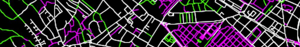
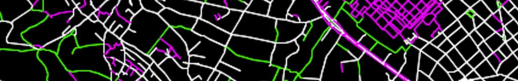
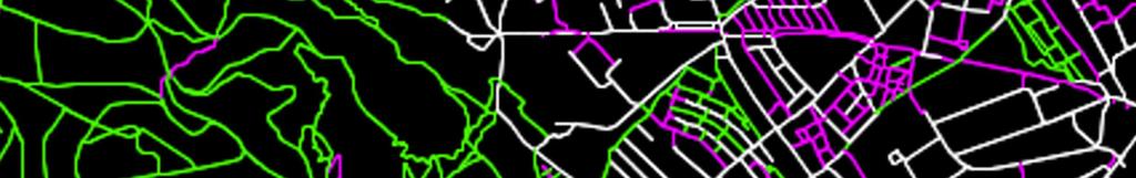
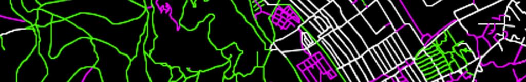
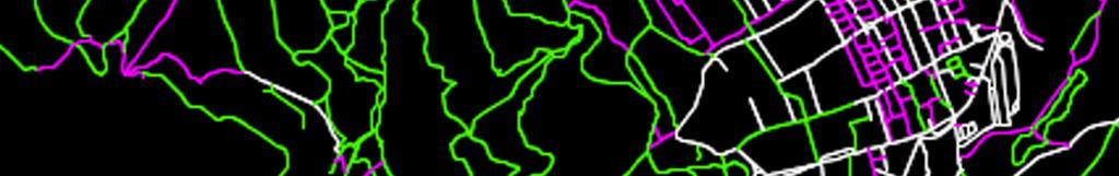
143 125